lmfit
前回、PythonのNumPyでリスト内の要素で条件に合った要素のインデックスを取得したり、置換するnp.whereを紹介しました。
今回はlmfitというライブラリを導入して、各種関数による分布の表示やピークフィッティングを行う方法を紹介します。
それでは始めていきましょう。
インストール
lmfitは外部ライブラリですので、使う前にはインストールが必要です。
インストールはpipでできます。
pip install lmfit分布の表示
まずはlmfitを使って、ガウス関数、ローレンツ関数、フォークト関数による分布を表示してみます。
これらの分布を表示するには「lmfit.lineshapes」の「gaussian」、「lorentzian」、「voigt」をインポートします。
まずはガウス関数による分布を見てみましょう。
ガウス関数の分布を取得するには「gaussian(X値のリスト, amplitude, center, sigma)」とします。
import numpy as np
import matplotlib.pyplot as plt
from lmfit.lineshapes import gaussian

x_list = np.arange(0, 100, 0.1)

y_gaussian = gaussian(x_list, 1, 50, 10)

fig = plt.figure()
plt.clf()

plt.plot(x_list, y_gaussian)

plt.show()

実行結果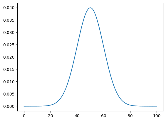
ローレンツ関数による分布の場合は「lorentzian(X値のリスト, amplitude, center, sigma)」とします。
import numpy as np
import matplotlib.pyplot as plt
from lmfit.lineshapes import lorentzian

x_list = np.arange(0, 100, 0.1)

y_lorentzian = lorentzian(x_list, 1, 50, 10)

fig = plt.figure()
plt.clf()

plt.plot(x_list, y_lorentzian)

plt.show()

実行結果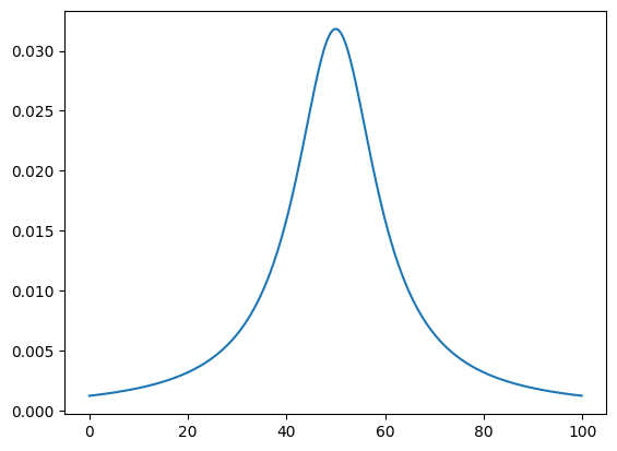
フォークと関数による分布の場合は「voigt(X値のリスト, amplitude, center, sigma, gamma)」とします。
import numpy as np
import matplotlib.pyplot as plt
from lmfit.lineshapes import voigt

x_list = np.arange(0, 100, 0.1)

y_voigt = voigt(x_list, 1, 50, 10, 2)

fig = plt.figure()
plt.clf()

plt.plot(x_list, y_voigt)

plt.show()

実行結果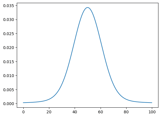
どんな関数が使用できるかはGitHubのページを見ると分かります。
フィッティングの仕方
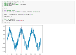
まずフィッティングを試すためのグラフを準備します。
今回は先ほど紹介したlmfitでガウス関数の取得方法を使って、そこにランダムな値を加減することでノイズを追加しました。
import numpy as np
import matplotlib.pyplot as plt
from lmfit.lineshapes import gaussian
from lmfit import models

rng = np.random.default_rng(123)

x_list = np.arange(0, 100, 0.1)

y_test = gaussian(x_list, 100, 50, 10) + rng.random(len(x_list)) - rng.random(len(x_list))

fig = plt.figure()
plt.clf()

plt.plot(x_list, y_test)

plt.show()

実行結果
ちなみにNumPyでジェネレータを使ったランダム値の取得方法はこちらの記事で紹介していますので、よかったらどうぞ。
これに対してフィッティングを行う場合、まずモデルを作成し、その次にそのモデルに対する初期パラメータを設定し、既知のY値と初期パラメータ、X値のリストを使ってフィッティングを行います。
今回、正解がガウス分布にノイズを加えたものと分かっているので、モデルをガウス関数とします。
また初期パラメータも答えが分かっているので、とりあえず設定してフィッティングをしてみます。
ということでフィッティングに必要な部分はこんな感じになります。
model = models.GaussianModel()
params = model.make_params(amplitude=100, center=50, sigma=10)
output = model.fit(y_test, params, x=x_list)
最初の行でモデルの設定、2行目の「model.make_params」でモデルに対してパラメータを設定、3行目の「model.fit」でフィッティングをしています。
ちなみにlmfitに含まれているモデルはこちらのページにまとめられています。
フィッティングの結果を数値で表示するにはmodel.fitの返り値に対して「.fit_report()」を用います。
import numpy as np
import matplotlib.pyplot as plt
from lmfit.lineshapes import gaussian
from lmfit import models

rng = np.random.default_rng(123)

x_list = np.arange(0, 100, 0.1)

y_test = gaussian(x_list, 100, 50, 10) + rng.random(len(x_list)) - rng.random(len(x_list))

model = models.GaussianModel()
params = model.make_params(amplitude=100, center=50, sigma=10)
output = model.fit(y_test, params, x=x_list)

print(output.fit_report())

実行結果
[[Model]]
    Model(gaussian)
[[Fit Statistics]]
    # fitting method   = leastsq
    # function evals   = 13
    # data points      = 1000
    # variables        = 3
    chi-square         = 169.188467
    reduced chi-square = 0.16969756
    Akaike info crit   = -1770.74199
    Bayesian info crit = -1756.01873
    R-squared          = 0.91824065
[[Variables]]
    amplitude:  101.679631 +/- 0.94709704 (0.93%) (init = 100)
    center:     49.8883264 +/- 0.10691622 (0.21%) (init = 50)
    sigma:      9.94065449 +/- 0.10691738 (1.08%) (init = 10)
    fwhm:       23.4084517 +/- 0.25177119 (1.08%) == '2.3548200*sigma'
    height:     4.08064744 +/- 0.03800934 (0.93%) == '0.3989423*amplitude/max(1e-15, sigma)'
[[Correlations]] (unreported correlations are < 0.100)
    C(amplitude, sigma) = +0.5774
フィッティングの結果をグラフとして表示する場合はmodel.fitの返り値に対して「.plot()」を用います。
import numpy as np
import matplotlib.pyplot as plt
from lmfit.lineshapes import gaussian
from lmfit import models

rng = np.random.default_rng(123)

x_list = np.arange(0, 100, 0.1)

y_test = gaussian(x_list, 100, 50, 10) + rng.random(len(x_list)) - rng.random(len(x_list))

model = models.GaussianModel()
params = model.make_params(amplitude=100, center=50, sigma=10)
output = model.fit(y_test, params, x=x_list)

fig = output.plot()

実行結果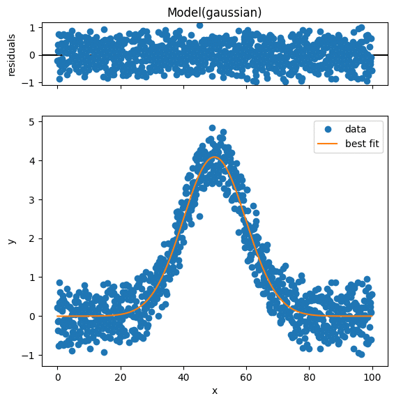
上のグラフが元のデータとフィッティング後のデータの残差を示していて、下のグラフが元のデータとフィッティング後のデータの比較となっています。
ちなみに「fig = output.plot()」という様に返り値を受け取らないとなぜかグラフが2回表示されるので注意してください。
グラフの表示形式を変える場合は「.plot()」に引数を与えます。
例えば「.plot(data_kws={“markersize”: 1})」とするとグラフの点のサイズが小さくなります。
import numpy as np
import matplotlib.pyplot as plt
from lmfit.lineshapes import gaussian
from lmfit import models

rng = np.random.default_rng(123)

x_list = np.arange(0, 100, 0.1)

y_test = gaussian(x_list, 100, 50, 10) + rng.random(len(x_list)) - rng.random(len(x_list))

model = models.GaussianModel()
params = model.make_params(amplitude=100, center=50, sigma=10)
output = model.fit(y_test, params, x=x_list)

fig = output.plot(data_kws={"markersize": 1})

実行結果
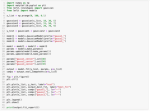
またベストフィットしたデータだけ欲しい場合はmodel.fitの返り値に対して「.best_fit」とするとフィッティング後のY値のリストが取得できます。
import numpy as np
import matplotlib.pyplot as plt
from lmfit.lineshapes import gaussian
from lmfit import models

rng = np.random.default_rng(123)

x_list = np.arange(0, 100, 0.1)

y_test = gaussian(x_list, 100, 50, 10) + rng.random(len(x_list)) - rng.random(len(x_list))

model = models.GaussianModel()
params = model.make_params(amplitude=100, center=50, sigma=10)
output = model.fit(y_test, params, x=x_list)

fig = plt.figure()
plt.clf()

plt.plot(x_list, y_test, label="data")
plt.plot(x_list, output.best_fit, label="best")

plt.legend()
plt.show()

実行結果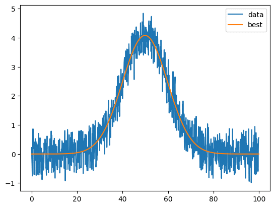
ベストフィットした際のパラメータが欲しい場合はmodel.fitの返り値に対して「.best_values」とするとフィッティング後のパラメータが取得できます。
import numpy as np
import matplotlib.pyplot as plt
from lmfit.lineshapes import gaussian
from lmfit import models

rng = np.random.default_rng(123)

x_list = np.arange(0, 100, 0.1)

y_test = gaussian(x_list, 100, 50, 10) + rng.random(len(x_list)) - rng.random(len(x_list))

model = models.GaussianModel()
params = model.make_params(amplitude=100, center=50, sigma=10)
output = model.fit(y_test, params, x=x_list)

print(output.best_values)

実行結果
{'amplitude': 101.67963063713268, 'center': 49.88832635569921,
'sigma': 9.940654491261505}
フィッティング精度を向上させる方法
フィッティング精度を向上させるには初期パラメータをなるべく正解に近い値で与えることが重要になります。
例えば先ほどのガウス関数のフィッティングの場合、初期パラメータを与えないと全くフィッティングに成功しません。
import numpy as np
import matplotlib.pyplot as plt
from lmfit.lineshapes import gaussian
from lmfit import models

rng = np.random.default_rng(123)

x_list = np.arange(0, 100, 0.1)

y_test = gaussian(x_list, 100, 50, 10) + rng.random(len(x_list)) - rng.random(len(x_list))

model = models.GaussianModel()
params = model.make_params()
output = model.fit(y_test, params, x=x_list)

fig = output.plot(data_kws={"markersize": 1})
print(output.best_values)

実行結果
{'amplitude': 0.22235321058106677, 'center': 0.6831262047971183,
'sigma': 0.1423961993828886}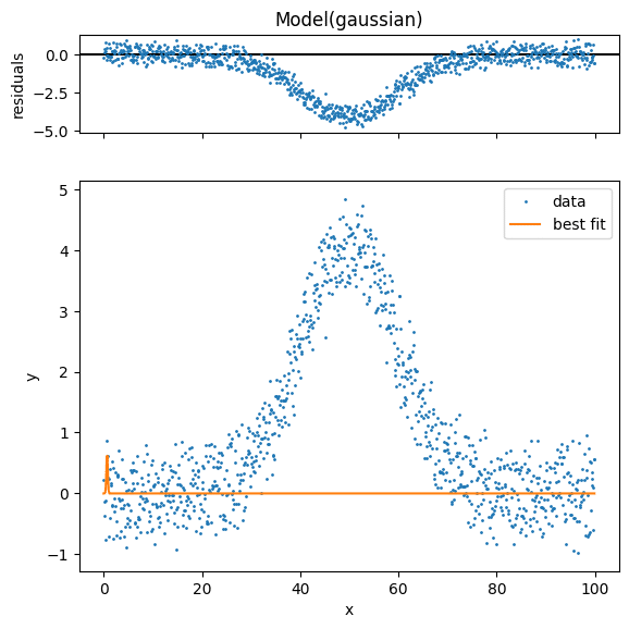
ガウス関数の場合これに頂点の位置(center)だけでも初期パラメータを与えるとフィッティングに成功しやすくなります。
import numpy as np
import matplotlib.pyplot as plt
from lmfit.lineshapes import gaussian
from lmfit import models

rng = np.random.default_rng(123)

x_list = np.arange(0, 100, 0.1)

y_test = gaussian(x_list, 100, 50, 10) + rng.random(len(x_list)) - rng.random(len(x_list))

model = models.GaussianModel()
params = model.make_params(center=50)
output = model.fit(y_test, params, x=x_list)

fig = output.plot(data_kws={"markersize": 1})
print(output.best_values)

実行結果
{'amplitude': 101.67963178291772, 'center': 49.8883263875762,
'sigma': 9.940654716217127}
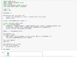
ピーク位置に関してはSciPyのfind_peaksを使うとピークの位置を取得することができます。
SciPyのcurve_fitの場合もピーク位置を与えることでフィッティング精度をあげることができました。
lmfitでも同じ方法を使ってもいいのですが、実はlmfitには初期パラメータを推測する様な関数「.guess」が準備されています。
モデル(model)を作成した後で「model.guess(既知のY値のリスト, X値のリスト)」とすることで大体の値を推測してくれます。
値の取得方法は「model.guessの返り値[“パラメータ名”].value」で取得できます。
import numpy as np
import matplotlib.pyplot as plt
from lmfit.lineshapes import gaussian
from lmfit import models

rng = np.random.default_rng(123)

x_list = np.arange(0, 100, 0.1)

y_test = gaussian(x_list, 100, 50, 10) + rng.random(len(x_list)) - rng.random(len(x_list))

model = models.GaussianModel()
guess = model.guess(y_test, x_list)

print(guess)
print(guess["amplitude"])
print(guess["amplitude"].value)

実行結果
Parameters([('amplitude', <Parameter 'amplitude', value=235.01838229298022,
bounds=[-inf:inf]>), ('center', <Parameter 'center', value=49.95690376569038,
bounds=[-inf:inf]>), ('sigma', <Parameter 'sigma', value=13.45,
bounds=[0.0:inf]>), ('fwhm', <Parameter 'fwhm', value=31.672329,
bounds=[-inf:inf], expr='2.3548200*sigma'>), ('height', <Parameter
'height', value=6.9709125631405815, bounds=[-inf:inf],
expr='0.3989423*amplitude/max(1e-15, sigma)'>)])
<Parameter 'amplitude', value=235.01838229298022, bounds=[-inf:inf]>
235.01838229298022
先ほどお話しした通りガウス関数ではピーク位置の情報を与えるだけでもフィッティング精度を上げられますので、ピーク位置「guess[“center”].value」だけ初期パラメータに与えてみます。
import numpy as np
import matplotlib.pyplot as plt
from lmfit.lineshapes import gaussian
from lmfit import models

rng = np.random.default_rng(123)

x_list = np.arange(0, 100, 0.1)

y_test = gaussian(x_list, 100, 50, 10) + rng.random(len(x_list)) - rng.random(len(x_list))

model = models.GaussianModel()
guess = model.guess(y_test, x_list)
params = model.make_params(center=guess["center"].value)
output = model.fit(y_test, params, x=x_list)

fig = output.plot(data_kws={"markersize": 1})
print(output.best_values)

実行結果
{'amplitude': 101.67963412204608,
 'center': 49.8883264839659,
 'sigma': 9.940655173216609}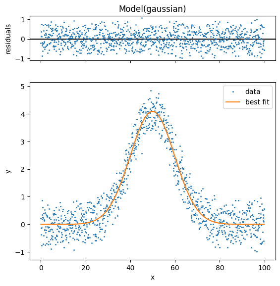
これで初期パラメータまで自動で設定し、ちゃんとフィッティングを行うことができました。
次回はlmfitを使って複数のピークに対してフィッティングをする方法を紹介します。
ではでは今回はこんな感じで。
コメント