lmfit
前回、Pythonのlmfitで複数のピークが混ざったグラフに対してピークフィッティングする方法を紹介しました。
今回は左右非対称のフォークト関数モデルSkewedVoigtModelを試してみます。
実は前に左右非対称のフォークト関数のモデルを自分で作成したこともあります。
せっかくなのでお手製の左右非対称のフォークト関数に対してSkewedVoigtModelでフィッティングしてみることにします。
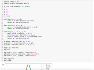
前に作成した左右非対称のフォークト関数モデルはこんな感じでした。
import numpy as np
import matplotlib.pyplot as plt
from lmfit.lineshapes import voigt

x_list_info = [0, 100, 0.1]

a = 1
mu = 50
sigma_L = 5
sigma_R = 10
gamma_L = 5
gamma_R = 10
ratio_1 = 0.3
ratio_2 = 0.7

def gauss(x, a, m, s):
    curve = np.exp(-(x-m)**2/(2*s**2))
    return a * curve/max(curve)

def lorentz(x, a, m, g):
    curve = (1/np.pi)*(g/((x-m)**2 + g**2))
    return a * curve/max(curve)

def voigt(x, a, m, s, g, r):
    gauss_curve = gauss(x, a, m, s)
    lorentz_curve = lorentz(x, a, m, g)
    curve = r*gauss_curve + (1-r)*lorentz_curve
    return a * curve/max(curve)

def asymmetric_voigt(x, a, m, s1, s2, g1, g2, r1, r2):
    peak_index = int(m / x_list_info[2])
    voigt_R = voigt(x, a, m, s1, g1, r1)
    voigt_L= voigt(x, a, m, s2, g2, r2)
    curve = np.concatenate([voigt_R[:peak_index], voigt_L[peak_index:]])
    return a * curve/max(curve)

x_list = np.arange(x_list_info[0], x_list_info[1], x_list_info[2])

y_asym_voigt = asymmetric_voigt(x_list, a, mu, sigma_L, sigma_R, gamma_L, gamma_R, ratio_1, ratio_2)

fig = plt.figure()
plt.clf()

plt.plot(x_list, y_asym_voigt)

plt.show()

実行結果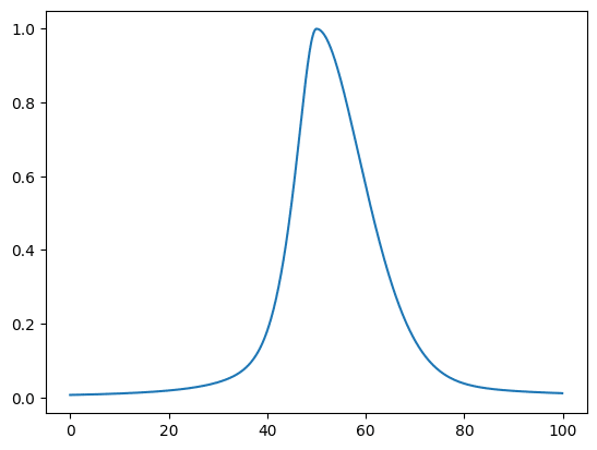
それでは始めていきましょう。
SkewedVoigtModelでフィッティング
まずはSkewedVoigtModelで自作の左右非対称のフォークト関数をフィッティングしてみます。
今回はSkewedVoigtModelを使うのでこんな感じです。
import numpy as np
import matplotlib.pyplot as plt
from lmfit.lineshapes import voigt
from lmfit import models

x_list_info = [0, 100, 0.1]

a = 1
mu = 50
sigma_L = 5
sigma_R = 10
gamma_L = 5
gamma_R = 10
ratio_1 = 0.3
ratio_2 = 0.7

def gauss(x, a, m, s):
    curve = np.exp(-(x-m)**2/(2*s**2))
    return a * curve/max(curve)

def lorentz(x, a, m, g):
    curve = (1/np.pi)*(g/((x-m)**2 + g**2))
    return a * curve/max(curve)

def voigt(x, a, m, s, g, r):
    gauss_curve = gauss(x, a, m, s)
    lorentz_curve = lorentz(x, a, m, g)
    curve = r*gauss_curve + (1-r)*lorentz_curve
    return a * curve/max(curve)

def asymmetric_voigt(x, a, m, s1, s2, g1, g2, r1, r2):
    peak_index = int(m / x_list_info[2])
    voigt_R = voigt(x, a, m, s1, g1, r1)
    voigt_L= voigt(x, a, m, s2, g2, r2)
    curve = np.concatenate([voigt_R[:peak_index], voigt_L[peak_index:]])
    return a * curve/max(curve)

x_list = np.arange(x_list_info[0], x_list_info[1], x_list_info[2])

y_asym_voigt = asymmetric_voigt(x_list, a, mu, sigma_L, sigma_R, gamma_L, gamma_R, ratio_1, ratio_2)

model = models.SkewedVoigtModel()
params = model.make_params()
output = model.fit(y_asym_voigt, params, x=x_list)

fig = output.plot(data_kws={"markersize": 1})
print(output.fit_report())

実行結果
[[Model]]
    Model(skewed_voigt)
[[Fit Statistics]]
    # fitting method   = leastsq
    # function evals   = 249
    # data points      = 1000
    # variables        = 4
    chi-square         = 0.66282894
    reduced chi-square = 6.6549e-04
    Akaike info crit   = -7310.99362
    Bayesian info crit = -7291.36259
    R-squared          = 0.99227253
[[Variables]]
    amplitude:  21.1785078 +/- 0.06416510 (0.30%) (init = 1)
    center:     49.2114964 +/- 0.16261770 (0.33%) (init = 0)
    sigma:      4.84927471 +/- 0.04923213 (1.02%) (init = 1)
    skew:       0.39675552 +/- 0.02408774 (6.07%) (init = 0)
    gamma:      4.84927471 +/- 0.04923213 (1.02%) == 'sigma'
[[Correlations]] (unreported correlations are < 0.100)
    C(center, skew)     = -0.9880
    C(center, sigma)    = -0.9291
    C(sigma, skew)      = +0.9246
    C(amplitude, sigma) = +0.1540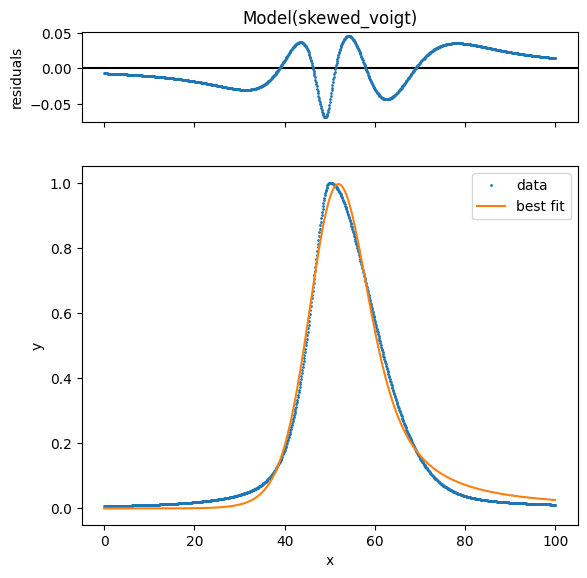
思ったよりもズレていたので、やはり自分でこういった関数を作る際にはちゃんとした知識が必要だと痛感しました。
フィッティングの結果を見てみると分かる様にSkewedVoigtModelでは「amplitude」、「center」、「sigma」、「skew」、「gamma」の5つのパラメータを用いています。
SkewedVoigtModelを描いてみる
次にSkewedVoigtModelにパラメーターを与えてグラフとして描いてみます。
ここで気をつけることは関数名とパラメータの順番です。
SkewedVoigtModelを描く際の関数は「lmfit.lineshapes」の「skewed_voigt」です。
引数に与えるパラメーターの順番を確認するにはhelp関数を使うのがいいです。
help(skewed_voigt)

実行結果
Help on function skewed_voigt in module lmfit.lineshapes:

skewed_voigt(x, amplitude=1.0, center=0.0, sigma=1.0, gamma=None, skew=0.0)
    Return a Voigt lineshape, skewed with error function.

    Equal to: voigt(x, center, sigma, gamma)*(1+erf(beta*(x-center)))

    where ``beta = skew/(sigma*sqrt(2))``

    with ``skew < 0``: tail to low value of centroid
         ``skew > 0``: tail to high value of centroid

    Useful, for example, for ad-hoc Compton scatter profile. For more
    information, see: https://en.wikipedia.org/wiki/Skew_normal_distribution
先ほどフィッティングの結果では「amplitude」、「center」、「sigma」、「skew」、「gamma」の順番で値が出力されていましたが、skewed_voigt関数では「amplitude」、「center」、「sigma」、「gamma」、「skew」の順番となっています。
もちろんこの順番を間違えると予想したグラフとは違うものが出てきますので注意しましょう。
先ほどフィッティングで得られたパラメータをskewed_voigt関数に与えてみましょう。
import numpy as np
import matplotlib.pyplot as plt
from lmfit.lineshapes import skewed_voigt

x_list = np.arange(0, 100, 0.1)

y_skewedvoigt = skewed_voigt(x_list, 26.63, 45.35, 8.46, 8.46, 1.64)

fig = plt.figure()
plt.clf()

plt.plot(x_list, y_skewedvoigt)

plt.show()

実行結果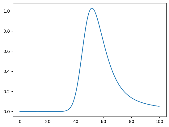
次回はもう一度SciPyのcurve_fitに戻ってパラメータの範囲の与え方を紹介します。
ではでは今回はこんな感じで。
コメント