NumPy
前回、Randomモジュール、NumPy、SciPyでランダムな値を取得する際のランダム(乱数)シードの設定方法を紹介しました。
今回はNumPyで多項式のカーブフィッティングをする関数polyfitを紹介します。
それでは始めていきましょう。
polyfit
polyfitを使うには「numpy」をインポートし、「np.polyfit(判明しているX値, 判明しているY値, 次数)」で使用できます。
返り値として次数にあった係数、例えば1次関数なら\(y = ax + b\)のため係数はa、bの2つ、2次関数なら\(y = ax^2 + bx + c\)のため係数は3つ、3次関数なら\(y = ax^3 + bx^2 + cx + d\)のため係数はa、b、c、dの4つになります。
ということで1次関数の場合はこんな感じです。
import numpy as np
import matplotlib.pyplot as plt

a = 2
b = 5

x_list = np.arange(-10, 10, 0.1)
y_list = [a*x + b for x in x_list]

estimate = np.polyfit(x_list, y_list, 1)
print(estimate)

y_estimate_list = [estimate[0]*x + estimate[1] for x in x_list]


fig = plt.figure()
plt.clf()

plt.plot(x_list, y_estimate_list, color="tab:orange", lw=3)
plt.plot(x_list, y_list, ls="--", color="tab:blue")

plt.show()

実行結果
[2. 5.]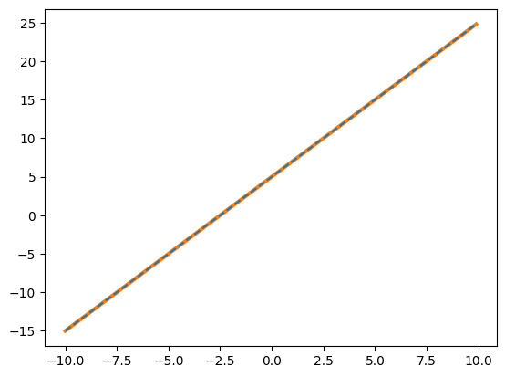
元のデータを青の点線で、polyfitでフィッティングした結果が橙色の線です。
フィッテングにより算出した係数を表示していますが、最初に入力した値(a = 2、b = 5)と同じ値になっています。
次に2次関数と3次関数の例です。
import numpy as np
import matplotlib.pyplot as plt

a = 2
b = 5
c = 10

x_list = np.arange(-10, 10, 0.1)
y_list = [a*x**2 + b*x + c  for x in x_list]

estimate = np.polyfit(x_list, y_list, 2)
print(estimate)

y_estimate_list = [estimate[0]*x**2 + estimate[1]*x + estimate[2] for x in x_list]


fig = plt.figure()
plt.clf()

plt.plot(x_list, y_estimate_list, color="tab:orange", lw=3)
plt.plot(x_list, y_list, ls="--", color="tab:blue")

plt.show()

実行結果
[ 2.  5. 10.]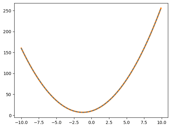
import numpy as np
import matplotlib.pyplot as plt

a = 2
b = 5
c = 10
d = 3

x_list = np.arange(-10, 10, 0.1)
y_list = [a*x**3 + b*x**2 + c*x + d  for x in x_list]

estimate = np.polyfit(x_list, y_list, 3)
print(estimate)

y_estimate_list = [estimate[0]*x**3 + estimate[1]*x**2 + estimate[2]*x + estimate[3] for x in x_list]


fig = plt.figure()
plt.clf()

plt.plot(x_list, y_estimate_list, color="tab:orange", lw=3)
plt.plot(x_list, y_list, ls="--", color="tab:blue")

plt.show()

実行結果
[ 2.  5. 10.  3.]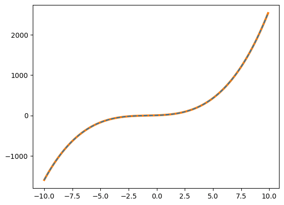
2次関数でも3次関数でも元のデータがノイズのない綺麗なデータの場合、間違えずにフィッティングをしてくれます。
次数が間違っている場合
ただしフィッティングする関数の次数と指定した次数が異なる場合はフィッティング結果が大きくずれてしまう可能性があることに注意してください。
例えば3次関数を2次関数と見誤りフィッティングするとこうなります。
import numpy as np
import matplotlib.pyplot as plt

a = 2
b = 5
c = 10
d = 3

x_list = np.arange(-10, 10, 0.1)
y_list = [a*x**3 + b*x**2 + c*x + d  for x in x_list]

estimate = np.polyfit(x_list, y_list, 2)
print(estimate)

y_estimate_list = [estimate[0]*x**2 + estimate[1]*x + estimate[2] for x in x_list]


fig = plt.figure()
plt.clf()

plt.plot(x_list, y_estimate_list, color="tab:orange", lw=3)
plt.plot(x_list, y_list, ls="--", color="tab:blue")

plt.show()

実行結果
[  4.7    129.978    8.9994]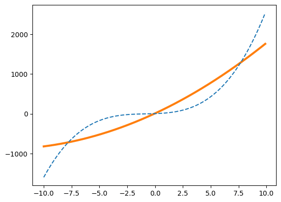
ただし元の関数の次数よりフィッティングのため指定した関数の次数の方が大きい場合は綺麗にフィッティングできてしまう場合もあります。
例えば3次関数を5次関数としてフィッティングするとこうなります。
import numpy as np
import matplotlib.pyplot as plt

a = 2
b = 5
c = 10
d = 3

x_list = np.arange(-10, 10, 0.1)
y_list = [a*x**3 + b*x**2 + c*x + d  for x in x_list]

estimate = np.polyfit(x_list, y_list, 5)
print(estimate)

y_estimate_list = [estimate[0]*x**5 + estimate[1]*x**4 + estimate[2]*x**3 + estimate[3]*x**2 + estimate[4]*x + estimate[5] for x in x_list]


fig = plt.figure()
plt.clf()

plt.plot(x_list, y_estimate_list, color="tab:orange", lw=3)
plt.plot(x_list, y_list, ls="--", color="tab:blue")

plt.show()

実行結果
[ 1.92932863e-18 -1.54300089e-16  2.00000000e+00  5.00000000e+00
  1.00000000e+01  3.00000000e+00]
この場合、最初の2つの係数がほぼ0であるため、係数をしっかりと確認すれば3次関数であることが分かります。
実際の利用例
実際にはノイズが入ったデータに対しフィッティングをすると思われます。
例えば2次関数にノイズをのせたデータを例にフィッティングしてみましょう。
import numpy as np
import matplotlib.pyplot as plt

a = 2
b = 5
c = 10

x_list = np.arange(-10, 10, 0.1)
y_list = [a*x**2 + b*x + c + np.random.uniform(-50, 50) for x in x_list]

estimate = np.polyfit(x_list, y_list, 2)
print(estimate)

y_estimate_list = [estimate[0]*x**2 + estimate[1]*x + c  for x in x_list]


fig = plt.figure()
plt.clf()

plt.plot(x_list, y_estimate_list, color="tab:orange", lw=3)
plt.scatter(x_list, y_list, ls="--", color="tab:blue")

plt.show()

実行結果
[2.09183185 5.67465293 9.31259666]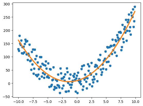
残差平方和(RSS: residual sum of squares)
今回はフィッティングに用いるデータを自分で作成してからフィッティングを行いました。
そのためそれぞれの係数を知っているため、フィッティング結果がどれくらい正確か一目瞭然でした。
しかしながら現実のデータはどんな係数なのか、はたまた何次の関数なのか分からない状態でフィッティングを行います。
先ほどの様に係数やグラフを確認することである程度わかることもあるのですが、どれくらいフィッティング結果がデータにフィットしているのかを知りたい場合もあることでしょう。
その際の一つの指標としてpolyfitでは残差平方和を算出することができます。
残差平方和は各点において実際の値とフィッティングした値を引き算し、2乗したものを足し合わせたものになります。
そのため値が小さいほど実際の値とフィッティングした値が近いという指標になります。
その場合は「np.polyfit()」のオプションとして「full=True」を追加します。
「full=True」のオプションを追加した場合、返り値に係数だけでなく色々なものが含まれるようになるので注意してください。
2次関数を例にして試してみましょう。
import numpy as np
import matplotlib.pyplot as plt

a = 2
b = 5
c = 10

x_list = np.arange(-10, 10, 0.1)
y_list = [a*x**2 + b*x + c  for x in x_list]

fitting_results = np.polyfit(x_list, y_list, 2, full=True)
print(fitting_results)

estimate = fitting_results[0]

y_estimate_list = [estimate[0]*x**2 + estimate[1]*x + estimate[2] for x in x_list]


fig = plt.figure()
plt.clf()

plt.plot(x_list, y_estimate_list, color="tab:orange", lw=3)
plt.plot(x_list, y_list, ls="--", color="tab:blue")

plt.show()

実行結果
(array([ 2.,  5., 10.]), array([1.33319949e-25]), 3,
array([1.32130905, 0.99977518, 0.50457109]), 4.440892098500626e-14)
表示された2番目の数値が残差平方和です。
次に2次関数にノイズをのせたデータで試してみましょう。
import numpy as np
import matplotlib.pyplot as plt

a = 2
b = 5
c = 10

x_list = np.arange(-10, 10, 0.1)
y_list = [a*x**2 + b*x + c + np.random.uniform(-50, 50) for x in x_list]

fitting_results = np.polyfit(x_list, y_list, 2, full=True)
print(fitting_results)

estimate = fitting_results[0]

y_estimate_list = [estimate[0]*x**2 + estimate[1]*x + c  for x in x_list]


fig = plt.figure()
plt.clf()

plt.plot(x_list, y_estimate_list, color="tab:orange", lw=3)
plt.scatter(x_list, y_list, ls="--", color="tab:blue")

plt.show()

実行結果
(array([ 1.99764926,  4.74644389, 12.45510034]),
array([151128.13980061]), 3, array([1.32130905, 0.99977518,
0.50457109]), 4.440892098500626e-14)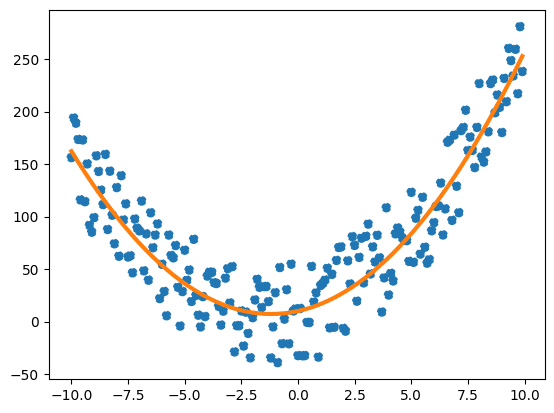
ピッタリ合っている最初の例では残差平方和は「1.33319949e-25」とかなり小さくなります。
しかしノイズが含まれている様な2番目の例の残差平方和は「18279314.84570362」と大きくなります。
ただしあくまでも元のデータとフィッティングしたデータが近ければ小さくなるという性質のものであり、いくつ以上になったら間違っているという性質のものではないことに注意してください。
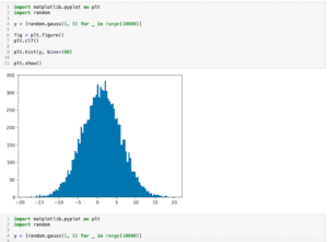
次回はmatplotlibでヒストグラムを表示する関数「hist」を紹介します。
ではでは今回はこんな感じで。
コメント