NumPy
前回、itertoolsのdropwhile、takewhile、filterfalse、starmapの使い方を紹介しました。
今回はNumPyを使って任意の平均・標準誤差をもつガウス分布(正規分布)を作る方法を紹介します。
それでは始めていきましょう。
ジェネレータを使う方法
まずはジェネレータを使い、その中の正規分布の乱数である「normal」を使って任意の平均・標準誤差をもつガウス分布(正規分布)を作ってみましょう。
ちなみにNumPy randomモジュールのジェネレータの使い方はこちらの記事で解説していますので、よかったらどうぞ。
ジェネレータを使う場合は「rng = np.random.default_rng()」としてインスタンスを生成します。
そしてnormal(正規分布)を使う場合は「rng.normal(mu, sigma, サンプル数)」とします。
muは平均値、sigmaは標準誤差です。
import numpy as np
import matplotlib.pyplot as plt

samples = 100000

mu = 50
sigma = 5

rng = np.random.default_rng(0)

data = rng.normal(mu, sigma, samples)

fig = plt.figure()
plt.clf()

plt.hist(data, bins=100)

plt.show()

実行結果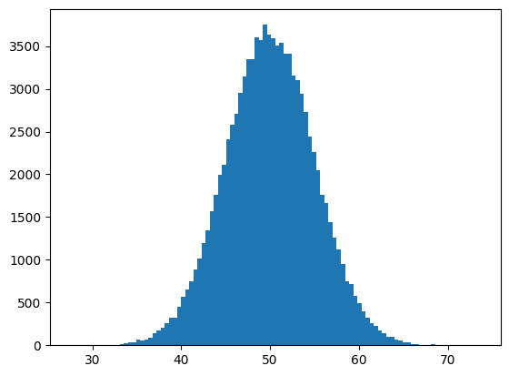
もしくは「mu + sigma * rng.normal(size=サンプル数)」とします。
import numpy as np
import matplotlib.pyplot as plt

samples = 100000

mu = 50
sigma = 5

rng = np.random.default_rng(0)

data = mu + sigma * rng.normal(size=samples)

fig = plt.figure()
plt.clf()

plt.hist(data, bins=100)

plt.show()

実行結果
ジェネレータを使う場合、もう一つ「rng.standard_normal(サンプル数)」も使うことができます。
こちらは平均0、 標準偏差1の正規分布の乱数を生成する関数です。
そのためmuとsigmaを引数には取れず、サンプル数のみを取りますので、ご注意ください。
つまり「mu + sigma * rng.standard_normal(サンプル数)」のみ使うことができます。
import numpy as np
import matplotlib.pyplot as plt

samples = 100000

mu = 50
sigma = 5

rng = np.random.default_rng(0)

data = mu + sigma * rng.standard_normal(samples)

fig = plt.figure()
plt.clf()

plt.hist(data, bins=100)

plt.show()

実行結果
np.random.normalを使う方法
またジェネレータと使わない場合の、rng.normalと同じ関数は「np.random.normal」です。
rng.normalと全く同じ使い方ができ、「np.random.normal(mu, sigma, サンプル数)」でも「mu + sigma * np.random.normal(size=samples)」でも使えます。
import numpy as np
import matplotlib.pyplot as plt

samples = 100000

mu = 50
sigma = 5

data = np.random.normal(mu, sigma, samples)

fig = plt.figure()
plt.clf()

plt.hist(data, bins=100)

plt.show()

実行結果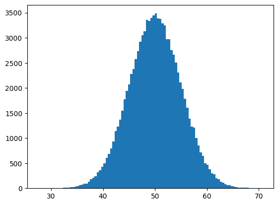
import numpy as np
import matplotlib.pyplot as plt

samples = 100000

mu = 50
sigma = 5

data = mu + sigma * np.random.normal(size=samples)

fig = plt.figure()
plt.clf()

plt.hist(data, bins=100)

plt.show()

実行結果
また「rng.standard_normal(サンプル数)」に当たるものが「np.random.randn(サンプル数)」です。
import numpy as np
import matplotlib.pyplot as plt

samples = 100000

mu = 50
sigma = 5

data = mu + sigma * np.random.randn(samples)

fig = plt.figure()
plt.clf()

plt.hist(data, bins=100)

plt.show()

実行結果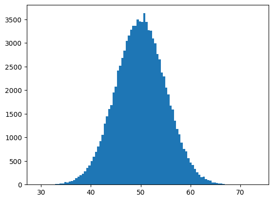
今回は任意の平均・標準誤差をもつガウス分布(正規分布)を作る方法として、ジェネレータを使う方法、使わない方法を紹介しました。
ただ今後は乱数を取得するのに、どうやらジェネレータを使う方が速く、今後主流になっていく様です。
ということでできる限りジェネレータを使って書く方に慣れていくのがいいでしょう。
次回はmatplotlibでバイオリンプロット(Violin Plot)を描く方法を紹介します。
ではでは今回はこんな感じで。
コメント