目次
Scikit-learn
前回、PythonのNumPyで多次元のndarrayやリストを一次元にする方法(.flatten、np.ravel)を紹介しました。
あわせて読みたい
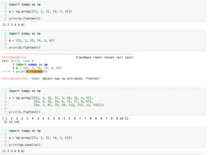
【NumPy】多次元のndarrayやリストを一次元にする方法(.flatten、np.ravel)[Python]
NumPy 前回、PythonのNumPyでndarrayをファイルに保存(np.save)、また読み込みする方法(np.load)を紹介しました。 今回はNumPyで多次元のndarrayやリストを一次元に…
今回はScikit-learnを使って二つのグラフの一致度を確認する方法を紹介します。
ということでまずは一致度を調べたいグラフを用意しました。
import numpy as np
import matplotlib.pyplot as plt
from scipy.optimize import curve_fit

x_list = np.arange(0, 100, 0.1)

a = 5
m = 50
s = 15

def gauss(x, a, m, s):
    curve = np.exp(-(x - m)**2/(2*s**2))
    return a * curve/max(curve)

rng = np.random.default_rng(123)

y_observed = gauss(x_list, a, m, s) + rng.random(len(x_list))

popt, pcov = curve_fit(gauss, x_list, y_observed, p0=[a, m, s])
y_estimate = gauss(x_list, popt[0], popt[1], popt[2])

fig = plt.figure()
plt.clf()

plt.plot(x_list, y_observed)
plt.plot(x_list, y_estimate)

plt.show()

実行結果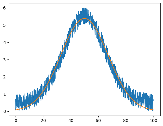
青色のグラフはガウス関数のグラフに乱数でノイズを加えたものです。
橙色のグラフは青色のグラフにSciPyのcurve_fitを使い、フィッティングしたものです。
それでは始めていきましょう。
決定係数R2を計算する方法
決定係数R2を計算するには「sklearn.metrics」の「r2_score」を使います。
使い方は「r2_score(グラフ1, グラフ2)」です。
Xの値は同じはずなので不要で、それぞれのYの値のリストだけを渡します。
import numpy as np
import matplotlib.pyplot as plt
from scipy.optimize import curve_fit
from sklearn.metrics import r2_score

x_list = np.arange(0, 100, 0.1)

a = 5
m = 50
s = 15

def gauss(x, a, m, s):
    curve = np.exp(-(x - m)**2/(2*s**2))
    return a * curve/max(curve)

rng = np.random.default_rng(123)

y_observed = gauss(x_list, a, m, s) + rng.random(len(x_list))

popt, pcov = curve_fit(gauss, x_list, y_observed, p0=[a, m, s])
y_estimate = gauss(x_list, popt[0], popt[1], popt[2])

r2 = r2_score(y_observed, y_estimate)

print(r2)

実行結果
0.9609991186694657
平均二乗誤差を計算する方法
平均二乗誤差を計算するには「sklearn.metrics」の「mean_squared_error」を用います。
使い方はr2_scoreと同じで「mean_squared_error(グラフ1, グラフ2)」です。
import numpy as np
import matplotlib.pyplot as plt
from scipy.optimize import curve_fit
from sklearn.metrics import mean_squared_error

x_list = np.arange(0, 100, 0.1)

a = 5
m = 50
s = 15

def gauss(x, a, m, s):
    curve = np.exp(-(x - m)**2/(2*s**2))
    return a * curve/max(curve)

rng = np.random.default_rng(123)

y_observed = gauss(x_list, a, m, s) + rng.random(len(x_list))

popt, pcov = curve_fit(gauss, x_list, y_observed, p0=[a, m, s])
y_estimate = gauss(x_list, popt[0], popt[1], popt[2])

mse = mean_squared_error(y_observed, y_estimate)

print(mse)

実行結果
0.12680740457390524
残差を表示する方法
視覚的にどこが違うかを知りたい場合は二つの差分である残差を計算、表示します。
import numpy as np
import matplotlib.pyplot as plt
from scipy.optimize import curve_fit
from sklearn.metrics import r2_score

x_list = np.arange(0, 100, 0.1)

a = 5
m = 50
s = 15

def gauss(x, a, m, s):
    curve = np.exp(-(x - m)**2/(2*s**2))
    return a * curve/max(curve)

rng = np.random.default_rng(123)

y_observed = gauss(x_list, a, m, s) + rng.random(len(x_list))

popt, pcov = curve_fit(gauss, x_list, y_observed, p0=[a, m, s])
y_estimate = gauss(x_list, popt[0], popt[1], popt[2])

y_residual = y_estimate - y_observed

fig = plt.figure()
plt.clf()

plt.plot(x_list, y_residual)

plt.axhline(0, c="gray", ls="--")

plt.show()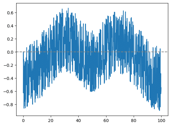
次回は自作関数を使ってガウス関数、ラプラス関数、ローレンツ関数を表示する方法を紹介します。
あわせて読みたい
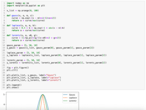
【matplotlib】ガウス分布、ラプラス分布、ローレンツ分布(コーシー分布)を自作関数化してグラフ表示…
matplotlib 前回、PythonのScikit-learnで二つのグラフの一致度を確認する方法を紹介しました。 今回はガウス分布、ラプラス分布、ローレンツ分布を自作関数化してグラ…
それでは今回はこんな感じで。
コメント