SciPy
前回、Pythonのlmfitで左右非対称のフォークト関数のモデルSkewedVoigtModelの使い方を紹介しました。
今回はSciPyのcurve_fitでパラメータの範囲を指定する方法を紹介します。
まず今回フィッティングさせる元のデータをガウス関数を使ってこんな感じに作ってみました。
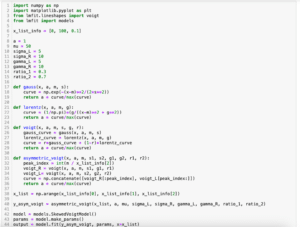
import numpy as np
import matplotlib.pyplot as plt
import random

x_min = 0
x_max = 100

def gauss(x_list, a=1, m=0, s=1):
    y_list = [a * np.exp(-(x - m)**2 / (2*s**2)) for x in x_list]
    return y_list

x_list = np.arange(x_min, x_max, 1)
y_list = gauss(x_list, 5, 50, 5)

fig = plt.figure()
plt.clf()

plt.scatter(x_list, y_list)

plt.show()

実行結果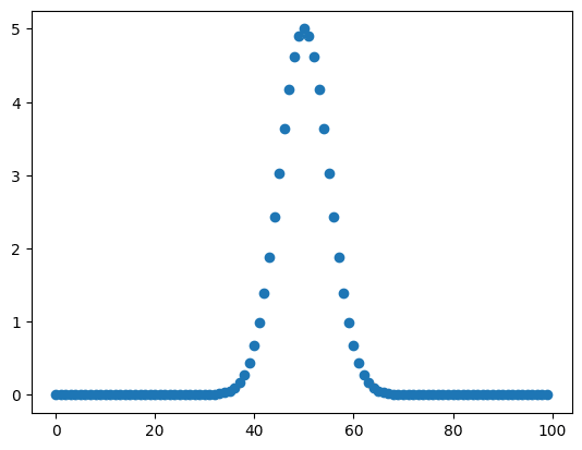
それでは始めていきましょう。
パラメータの範囲の与え方
まずはおさらいがてら初期パラメータもパラメータ範囲も与えずにcurve_fitしてみます。
import numpy as np
import matplotlib.pyplot as plt
import random
from scipy.optimize import curve_fit

x_min = 0
x_max = 100

def gauss(x_list, a=1, m=0, s=1):
    y_list = [a * np.exp(-(x - m)**2 / (2*s**2)) for x in x_list]
    return y_list

x_list = np.arange(x_min, x_max, 1)
y_list = gauss(x_list, 5, 50, 5)

popt, pcov = curve_fit(gauss, x_list, y_list)

fig = plt.figure()
plt.clf()

plt.scatter(x_list, y_list)
plt.plot(x_list, gauss(x_list, *popt))

plt.show()

実行結果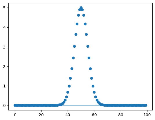
ピークに全くフィッティングできませんでした。
次に初期パラメータの与え方のおさらいとして、実際のパラメータとは少しずらしたパラメータを初期パラメータとして与えてみます。
初期パラメータはcurve_fitのオプション引数として「p0」を追加します。
import numpy as np
import matplotlib.pyplot as plt
import random
from scipy.optimize import curve_fit

x_min = 0
x_max = 100

initial_param = [3, 40, 7]

def gauss(x_list, a=1, m=0, s=1):
    y_list = [a * np.exp(-(x - m)**2 / (2*s**2)) for x in x_list]
    return y_list

x_list = np.arange(x_min, x_max, 1)
y_list = gauss(x_list, 5, 50, 5)

popt, pcov = curve_fit(gauss, x_list, y_list, p0=initial_param)

fig = plt.figure()
plt.clf()

plt.scatter(x_list, y_list)
plt.plot(x_list, gauss(x_list, *popt))

plt.show()

実行結果
しっかりフィッティングさせることができました。
次にパラメータの範囲を与えてフィッティングしてみます。
パラメータの範囲はcurve_fitのオプション引数として「bounds」を追加します。
またパラメータの範囲は「[[パラメータ1の最小値, パラメータ2の最小値, パラメータ3の最小値…], [パラメータ1の最大値, パラメータ2の最大値, パラメータ3の最大値…]]」のように、それぞれのパラメータの最小値のリスト、最大値のリストというようにまとめます。
import numpy as np
import matplotlib.pyplot as plt
import random
from scipy.optimize import curve_fit

x_min = 0
x_max = 100

bounds_params = [[0, 45, 0],[10, 55, 10]]

def gauss(x_list, a=1, m=0, s=1):
    y_list = [a * np.exp(-(x - m)**2 / (2*s**2)) for x in x_list]
    return y_list

x_list = np.arange(x_min, x_max, 1)
y_list = gauss(x_list, 5, 50, 5)

popt, pcov = curve_fit(gauss, x_list, y_list, bounds=bounds_params)

fig = plt.figure()
plt.clf()

plt.scatter(x_list, y_list)
plt.plot(x_list, gauss(x_list, *popt))

plt.show()

実行結果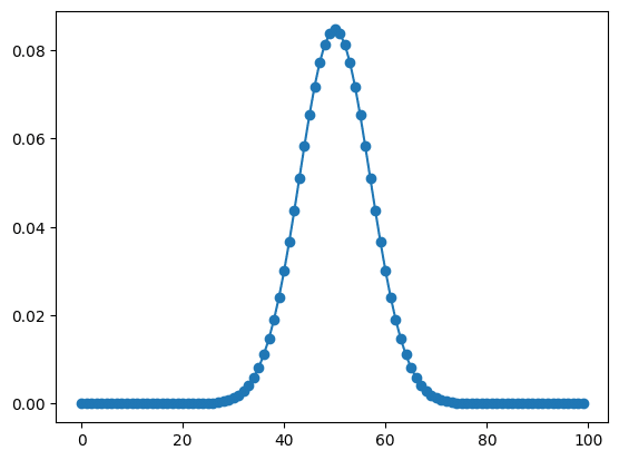
もちろん初期パラメータとパラメータ範囲を同時に与えることもできます。
import numpy as np
import matplotlib.pyplot as plt
import random
from scipy.optimize import curve_fit

x_min = 0
x_max = 100

initial_param = [5, 50, 5]
bounds_params = [[0, 45, 0],[10, 55, 10]]

def gauss(x_list, a=1, m=0, s=1):
    y_list = [a * np.exp(-(x - m)**2 / (2*s**2)) for x in x_list]
    return y_list

x_list = np.arange(x_min, x_max, 1)
y_list = gauss(x_list, 5, 50, 5)

popt, pcov = curve_fit(gauss, x_list, y_list, p0=initial_param, bounds=bounds_params)

fig = plt.figure()
plt.clf()

plt.scatter(x_list, y_list)
plt.plot(x_list, gauss(x_list, *popt))

plt.show()

実行結果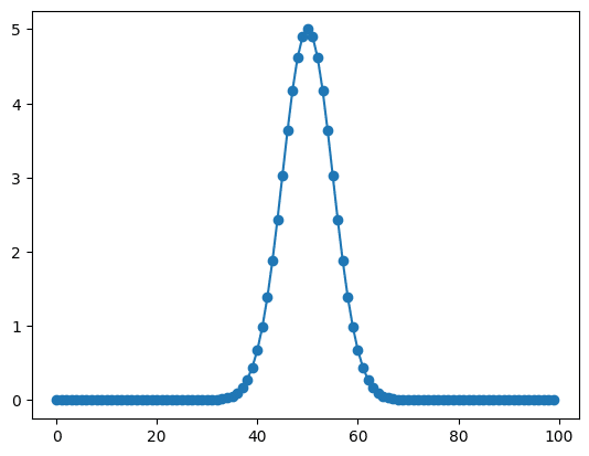
ただし初期パラメータとパラメータ範囲を両方与える場合、初期パラメータがパラメータ範囲外になっている場合エラーとなるので注意です。
import numpy as np
import matplotlib.pyplot as plt
import random
from scipy.optimize import curve_fit

x_min = 0
x_max = 100

initial_param = [20, 100, 20]
bounds_params = [[0, 45, 0],[10, 55, 10]]

def gauss(x_list, a=1, m=0, s=1):
    y_list = [a * np.exp(-(x - m)**2 / (2*s**2)) for x in x_list]
    return y_list

x_list = np.arange(x_min, x_max, 1)
y_list = gauss(x_list, 5, 50, 5)

popt, pcov = curve_fit(gauss, x_list, y_list, p0=initial_param, bounds=bounds_params)

fig = plt.figure()
plt.clf()

plt.scatter(x_list, y_list)
plt.plot(x_list, gauss(x_list, *popt))

plt.show()

実行結果
---------------------------------------------------------------------------
ValueError                                Traceback (most recent call last)
Cell In[8], line 19
     16 x_list = np.arange(x_min, x_max, 1)
     17 y_list = gauss(x_list, 5, 50, 5)
---> 19 popt, pcov = curve_fit(gauss, x_list, y_list, p0=initial_param, bounds=bounds_params)
     21 fig = plt.figure()
     22 plt.clf()

File /Library/Frameworks/Python.framework/Versions/3.10/lib/python3.10/site-packages/scipy/optimize/_minpack_py.py:974, in curve_fit(f, xdata, ydata, p0, sigma, absolute_sigma, check_finite, bounds, method, jac, full_output, nan_policy, **kwargs)
    971 if 'max_nfev' not in kwargs:
    972     kwargs['max_nfev'] = kwargs.pop('maxfev', None)
--> 974 res = least_squares(func, p0, jac=jac, bounds=bounds, method=method,
    975                     **kwargs)
    977 if not res.success:
    978     raise RuntimeError("Optimal parameters not found: " + res.message)

File /Library/Frameworks/Python.framework/Versions/3.10/lib/python3.10/site-packages/scipy/optimize/_lsq/least_squares.py:818, in least_squares(fun, x0, jac, bounds, method, ftol, xtol, gtol, x_scale, loss, f_scale, diff_step, tr_solver, tr_options, jac_sparsity, max_nfev, verbose, args, kwargs)
    814     raise ValueError("Each lower bound must be strictly less than each "
    815                      "upper bound.")
    817 if not in_bounds(x0, lb, ub):
--> 818     raise ValueError("`x0` is infeasible.")
    820 x_scale = check_x_scale(x_scale, x0)
    822 ftol, xtol, gtol = check_tolerance(ftol, xtol, gtol, method)

ValueError: `x0` is infeasible.
しかもこの場合のエラーメッセージは「 ‘x0’ is infeasible.」というだけで、詳細が書かれていないので、どんなエラーなのか分かりにくいです。
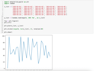
次回はmatplotlibで軸の値に特定の値を表示する方法、軸の値に文字列や日付を指定する方法を紹介します。
ではでは今回はこんな感じで。
コメント