機械学習ライブラリScikit-learn
前回まで機械学習ライブラリScikit-learnの生理学的データと運動能力の関係の分類のデータセットの紹介をしました。
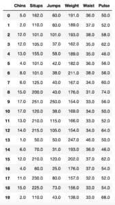
今回は最後の一つ「乳がん患者のデータセット」の紹介をしていきます。
それでは始めていきましょう。
データセットの読み込み
まずはデータセットの読み込みをしていきます。
今回も手間を省くため、オプションを「as_Frame = True」としてPandasのデータセット形式で読み込みます。
<セル1>

from sklearn.datasets import load_breast_cancer

cancer = load_breast_cancer(as_frame = True)

print(cancer.keys())

実行結果
dict_keys(['data', 'target', 'frame', 'target_names', 'DESCR', 'feature_names', 'filename'])
そしてデータを表示させてみます。
<セル2>

cancer.frame

実行結果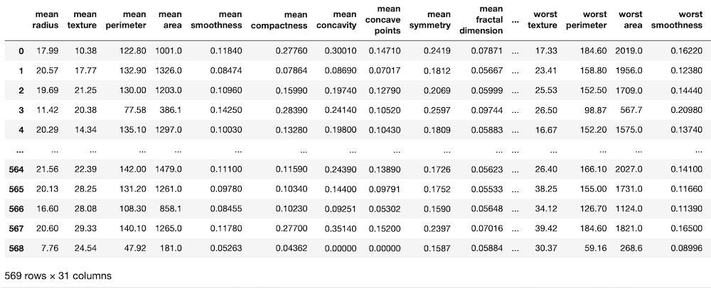
今回は特徴量が30もあるデータセットです。
こういうデータセットになるとどの特徴量を選ぶのかが重要になってきそうですね。
データセットの概要を確認
それではデータセットの概要を確認していきましょう。
<セル3>

.. _breast_cancer_dataset:

Breast cancer wisconsin (diagnostic) dataset
--------------------------------------------

**Data Set Characteristics:**

    :Number of Instances: 569

    :Number of Attributes: 30 numeric, predictive attributes and the class

    :Attribute Information:
        - radius (mean of distances from center to points on the perimeter)
        - texture (standard deviation of gray-scale values)
        - perimeter
        - area
        - smoothness (local variation in radius lengths)
        - compactness (perimeter^2 / area - 1.0)
        - concavity (severity of concave portions of the contour)
        - concave points (number of concave portions of the contour)
        - symmetry
        - fractal dimension ("coastline approximation" - 1)

        The mean, standard error, and "worst" or largest (mean of the three
        worst/largest values) of these features were computed for each image,
        resulting in 30 features.  For instance, field 0 is Mean Radius, field
        10 is Radius SE, field 20 is Worst Radius.

        - class:
                - WDBC-Malignant
                - WDBC-Benign

(以下略)
Number of Instances(データ数)は569、Number of Attributes(特徴量の数)は30です。
特徴量を一つずつ見ていきましょう。
radius:半径
texture:見た目(形状)
perimeter:境界線の状態
area:面積
smoothness:滑らかさ
compactness:コンパクト度(perimeter^2 / area – 1.0)
concavity:輪郭の凹部の重要度(凹部の強さ?)
concave points:凹部の数
symmetry:対称性
fractal dimension:フラクタル次元の数値
これらで特徴量が10個ですが、これらの数値に対し、mean(平均値)、standard error(標準誤差)、”worst”かlargest、つまり最悪か最大の状態、という3つの数値があり、そのため特徴量は30個となっています。
LinearRegressionで機械学習してみる
今回も回帰のデータセットになるので、LinearRegressionモデルを使って機械学習してみましょう。
<セル4>

from sklearn.linear_model import LinearRegression
from sklearn.model_selection import train_test_split
from sklearn.metrics import r2_score

x = cancer.frame.iloc[:, 0:-1]
y = cancer.frame.iloc[:, -1]

x_train, x_test, y_train, y_test = train_test_split(x, y, test_size=0.2, train_size=0.8)

model = LinearRegression()
model.fit(x_train, y_train)
pred = model.predict(x_test)

print(r2_score(y_test, pred))

実行結果
0.7566552520150847
予想スコアが0.75666ということで、なかなかいい値が出てきました。
先ほども少し言いましたが、特徴量の数が多いと言うことで、より特徴を掴んでいるものを選ぶことでもっと予想精度が上げられるのではないでしょうか。
またそれは気が向いたらやることにしましょう。
これで取り合えずScikit learnに含まれるデータセットは一旦終わりとしたいと思います。
次回からはもう少し実践的な事を試していきたいと考えています。
ではでは今回はこんな感じで。
コメント