Matplotlibで二次元リストを画像表示
前回、機械学習ライブラリScikit-learnの手書き数字のデータセットに含まれるデータを画像表示してみました。
そこでMatplotlibの中で二次元リストを画像表示する関数「matshow」を使いましたが、この関数が一体どういうものなのか今回はもう少し色々試してみたいと思います。
データは前回同様、Scikit-learnの手書き数字のデータセットのデータを使っていきます。
ということで読み込みから。
<セル1>

from sklearn.datasets import load_digits

digits = load_digits()

print(digits.data[0])

実行結果
[ 0.  0.  5. 13.  9.  1.  0.  0.  0.  0. 13. 15. 10. 15.  5.  0.  0.  3.
 15.  2.  0. 11.  8.  0.  0.  4. 12.  0.  0.  8.  8.  0.  0.  5.  8.  0.
  0.  9.  8.  0.  0.  4. 11.  0.  1. 12.  7.  0.  0.  2. 14.  5. 10. 12.
  0.  0.  0.  0.  6. 13. 10.  0.  0.  0.]
これでデータは読み込めました。
matshowのヘルプを確認
まずはmatshowのヘルプを見てみましょう。
<セル2>

import matplotlib.pyplot as plt

help(plt.matshow)

実行結果
Help on function matshow in module matplotlib.pyplot:

matshow(A, fignum=None, **kwargs)
    Display an array as a matrix in a new figure window.

    The origin is set at the upper left hand corner and rows (first
    dimension of the array) are displayed horizontally.  The aspect
    ratio of the figure window is that of the array, unless this would
    make an excessively short or narrow figure.

    Tick labels for the xaxis are placed on top.

    Parameters
    ----------
    A : array-like(M, N)
        The matrix to be displayed.

    fignum : None or int or False
        If *None*, create a new figure window with automatic numbering.

        If a nonzero integer, draw into the figure with the given number
        (create it if it does not exist).

        If 0, use the current axes (or create one if it does not exist).

        .. note::

           Because of how `.Axes.matshow` tries to set the figure aspect
           ratio to be the one of the array, strange things may happen if you
           reuse an existing figure.

    Returns
    -------
    image : `~matplotlib.image.AxesImage`

    Other Parameters
    ----------------
    **kwargs : `~matplotlib.axes.Axes.imshow` arguments
入力できるパラメータとしては3つ。
A:表示する二次元リスト
fignum:図の番号
**kwargs:これはよく分かりませんが、imshowを見れば分かるようです。
実はこの「matshow」という関数は「imshow」関数の簡易バージョンのようなものです。
ということで次回は「imshow」も見てみるということにしましょう。
今回はAとfignumがどういうパラメータなのかいじってみましょう。
A:表示する二次元リスト
Aには表示する二次元リストを入れます。
ということで前回使ったnumpyのreshapeを使って、同じデータから異なる二次元リストを作って、Aに入れてみましょう。
<セル3>

import numpy as np

data8_8 = np.reshape(digits.data[0], (8,8))
data4_16 = np.reshape(digits.data[0], (4,16))
data2_32 = np.reshape(digits.data[0], (2,32))

print(data8_8)
print(data4_16)
print(data2_32)

実行結果
[[ 0.  0.  5. 13.  9.  1.  0.  0.]
 [ 0.  0. 13. 15. 10. 15.  5.  0.]
 [ 0.  3. 15.  2.  0. 11.  8.  0.]
 [ 0.  4. 12.  0.  0.  8.  8.  0.]
 [ 0.  5.  8.  0.  0.  9.  8.  0.]
 [ 0.  4. 11.  0.  1. 12.  7.  0.]
 [ 0.  2. 14.  5. 10. 12.  0.  0.]
 [ 0.  0.  6. 13. 10.  0.  0.  0.]]
[[ 0.  0.  5. 13.  9.  1.  0.  0.  0.  0. 13. 15. 10. 15.  5.  0.]
 [ 0.  3. 15.  2.  0. 11.  8.  0.  0.  4. 12.  0.  0.  8.  8.  0.]
 [ 0.  5.  8.  0.  0.  9.  8.  0.  0.  4. 11.  0.  1. 12.  7.  0.]
 [ 0.  2. 14.  5. 10. 12.  0.  0.  0.  0.  6. 13. 10.  0.  0.  0.]]
[[ 0.  0.  5. 13.  9.  1.  0.  0.  0.  0. 13. 15. 10. 15.  5.  0.  0.  3.
  15.  2.  0. 11.  8.  0.  0.  4. 12.  0.  0.  8.  8.  0.]
 [ 0.  5.  8.  0.  0.  9.  8.  0.  0.  4. 11.  0.  1. 12.  7.  0.  0.  2.
  14.  5. 10. 12.  0.  0.  0.  0.  6. 13. 10.  0.  0.  0.]]
8×8、4×16、2×32の3種類の二次元リストを作ってみました。
それではそれぞれを画像表示してみます。
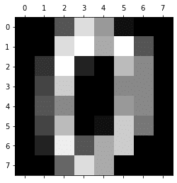
前回は「plt.gray()」でグレースケールにしましたが、今回は省略します。
また「plt.show()」でグラフ表示をしていたのですが、どうやらAnacondaを使っている状態ではなくても画像表示してくれるようなので、こちらも省略します。
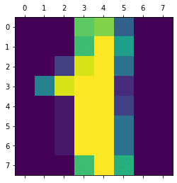
<セル4>

plt.matshow(data8_8)

実行結果
<セル5>

plt.matshow(data4_16)

実行結果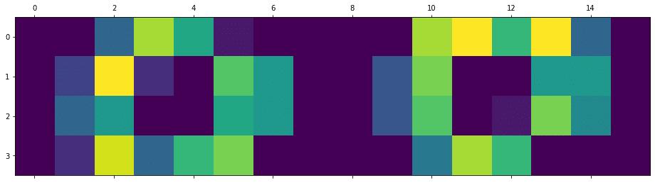
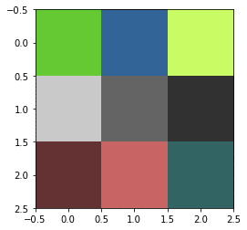
<セル6>

plt.matshow(data2_32)

実行結果
色はグレースケールにしないと緑、黄色と言った色で出るんですね。
ちなみに上の例では縦横の全てに数値が入っている綺麗な二次元リストですが、数値が欠けていたらどうなるのでしょうか?
ということで上の行から3個、3個、2個のデータを含んだリストを作成して試してみましょう。
<セル7>

data_num = [[2, 3, 5], [1, 4, 3], [4, 2]]

plt.matshow(data_num)

実行結果
---------------------------------------------------------------------------
ValueError                                Traceback (most recent call last)
<ipython-input-14-1b0d7b1eb16c> in <module>
      1 data_num = [[2, 3, 5], [1, 4, 3], [4, 2]]
      2
----> 3 plt.matshow(data_num)

/opt/anaconda3/lib/python3.7/site-packages/matplotlib/pyplot.py in matshow(A, fignum, **kwargs)
   2112         # Extract actual aspect ratio of array and make appropriately sized
   2113         # figure.
-> 2114         fig = figure(fignum, figsize=figaspect(A))
   2115         ax = fig.add_axes([0.15, 0.09, 0.775, 0.775])
   2116     im = ax.matshow(A, **kwargs)

/opt/anaconda3/lib/python3.7/site-packages/matplotlib/figure.py in figaspect(arg)
   2761     # Extract the aspect ratio of the array
   2762     if isarray:
-> 2763         nr, nc = arg.shape[:2]
   2764         arr_ratio = nr / nc
   2765     else:

ValueError: not enough values to unpack (expected 2, got 1)
縦横の数はあっていないとエラーとなるようです。
fignum:図の番号
次はfignum:図の番号です。
こちらは最初よく分からなかったのですが、複数の図を表示する時に使うオプションのようです。
reshapeするのは面倒なので、digits.imagesに含まれるデータで試してみましょう。
<セル8>

print(digits.images[0])
print(digits.images[1])
print(digits.images[2])

実行結果
[[ 0.  0.  5. 13.  9.  1.  0.  0.]
 [ 0.  0. 13. 15. 10. 15.  5.  0.]
 [ 0.  3. 15.  2.  0. 11.  8.  0.]
 [ 0.  4. 12.  0.  0.  8.  8.  0.]
 [ 0.  5.  8.  0.  0.  9.  8.  0.]
 [ 0.  4. 11.  0.  1. 12.  7.  0.]
 [ 0.  2. 14.  5. 10. 12.  0.  0.]
 [ 0.  0.  6. 13. 10.  0.  0.  0.]]
[[ 0.  0.  0. 12. 13.  5.  0.  0.]
 [ 0.  0.  0. 11. 16.  9.  0.  0.]
 [ 0.  0.  3. 15. 16.  6.  0.  0.]
 [ 0.  7. 15. 16. 16.  2.  0.  0.]
 [ 0.  0.  1. 16. 16.  3.  0.  0.]
 [ 0.  0.  1. 16. 16.  6.  0.  0.]
 [ 0.  0.  1. 16. 16.  6.  0.  0.]
 [ 0.  0.  0. 11. 16. 10.  0.  0.]]
[[ 0.  0.  0.  4. 15. 12.  0.  0.]
 [ 0.  0.  3. 16. 15. 14.  0.  0.]
 [ 0.  0.  8. 13.  8. 16.  0.  0.]
 [ 0.  0.  1.  6. 15. 11.  0.  0.]
 [ 0.  1.  8. 13. 15.  1.  0.  0.]
 [ 0.  9. 16. 16.  5.  0.  0.  0.]
 [ 0.  3. 13. 16. 16. 11.  5.  0.]
 [ 0.  0.  0.  3. 11. 16.  9.  0.]]
この三つの二次元リストを表示してみます。
まずはfignumのオプションなし。
<セル9>

plt.matshow(digits.images[0])
plt.matshow(digits.images[1])
plt.matshow(digits.images[2])

実行結果


入力した順番に画像が表示されました。
次にfignumのオプションを追加してみます。
先ほどのヘルプによると0は特殊なようなので、1から試してみます。
<セル10>

plt.matshow(digits.images[0], fignum=3)
plt.matshow(digits.images[1], fignum=2)
plt.matshow(digits.images[2], fignum=1)

実行結果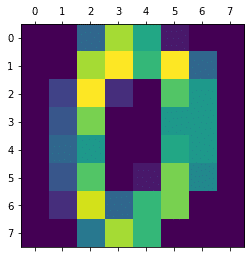


図の番号だから指定した順番に表示されると思ったのですが、どうもそうではないようです。
もしかしたら他のセルのデータを引きずっている可能性も考えられるので、先頭に「plt.clf()」をつけて、グラフエリアをリフレッシュしてから表示させてみましょう。
<セル11>
plt.clf()
plt.matshow(digits.images[0], fignum=3)
plt.matshow(digits.images[1], fignum=2)
plt.matshow(digits.images[2], fignum=1)

実行結果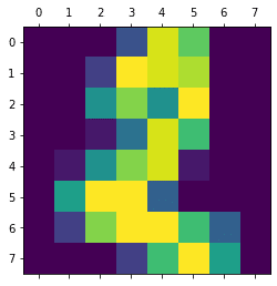

順番は変わったのですが、図の番号の指定は、2が1番、1が2番、0が3番としたのですが、そのとうりにはなっていません。
なかなか謎ですね。
多分、この後グラフをいじる時にこの番号を指定することで一つのグラフのみをいじることができるのではないかなと思われます。
次に3つのデータのfignumに0を指定してみましょう。
<セル12>

plt.matshow(digits.images[0], fignum=0)
plt.matshow(digits.images[1], fignum=0)
plt.matshow(digits.images[2], fignum=0)

実行結果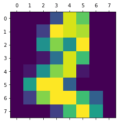
今度は2しか表示されませんでした。
多分同じ番号を指定したので、全て重なっていて、最後に描写された2が見えているのだと考えられます。
いうことで0のfignumを0、1のfignumを1、2のfignumを2としてみましょう。
<セル13>

plt.matshow(digits.images[0], fignum=0)
plt.matshow(digits.images[1], fignum=1)
plt.matshow(digits.images[2], fignum=2)

実行結果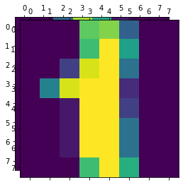

1の画像のところに少しずれてもう一枚、多分0の図が見えているようです。
fignumの0と1は同じものではないけども、同じ場所に表示されるということで、このように被って表示されてしまったと考えられます。
とりあえずfignumは使ってみたところ、図を指定して何かやらない限りは指定する必要はないのかなと感じました。
matshowの解説はこれくらいですが、次回はmatshowの元である関数「imshow」を見ていきたいと思います。
ということで今回はこんな感じで。
コメント