Matplotlibで二次元リストを画像表示
前回、Matplotlibライブラリのmatshowの解説をしました。
今回はその元となった関数「imshow」の解説を行っていきたいと思います。
ただこのimshowは結構色々なオプションがあるので、使いそうなものや私が試して理解できたものを何回かに分けて、解説することにします。
使うデータは前回同様、Scikit-learnに含まれる手書き数字のデータセットのデータを使います。
ということでまずは読み込みから。
今回はimagesの一番最初のデータを使っていくことにしましょう。
<セル1>

from sklearn.datasets import load_digits
import matplotlib.pyplot as plt

digits = load_digits()

print(digits.images[0])

実行結果
[[ 0.  0.  5. 13.  9.  1.  0.  0.]
 [ 0.  0. 13. 15. 10. 15.  5.  0.]
 [ 0.  3. 15.  2.  0. 11.  8.  0.]
 [ 0.  4. 12.  0.  0.  8.  8.  0.]
 [ 0.  5.  8.  0.  0.  9.  8.  0.]
 [ 0.  4. 11.  0.  1. 12.  7.  0.]
 [ 0.  2. 14.  5. 10. 12.  0.  0.]
 [ 0.  0.  6. 13. 10.  0.  0.  0.]]
今回はmatplotlibを使うのが分かっているので、最初のセルで読み込んでおくことにしました。
imshowのヘルプ
早速、imshowを使って画像表示をしていきたいところですが、最初にヘルプを確認しておきましょう。
<セル2>

help(plt.imshow)

実行結果
Help on function imshow in module matplotlib.pyplot:

imshow(X, cmap=None, norm=None, aspect=None, interpolation=None, alpha=None, vmin=None, vmax=None, origin=None, extent=None, shape=<deprecated parameter>, filternorm=1, filterrad=4.0, imlim=<deprecated parameter>, resample=None, url=None, *, data=None, **kwargs)

(中略)

    Parameters
    ----------
    X : array-like or PIL image
        The image data. Supported array shapes are:

        - (M, N): an image with scalar data. The values are mapped to
          colors using normalization and a colormap. See parameters *norm*,
          *cmap*, *vmin*, *vmax*.
        - (M, N, 3): an image with RGB values (0-1 float or 0-255 int).
        - (M, N, 4): an image with RGBA values (0-1 float or 0-255 int),
          i.e. including transparency.

        The first two dimensions (M, N) define the rows and columns of
        the image.

        Out-of-range RGB(A) values are clipped.

    cmap : str or `~matplotlib.colors.Colormap`, optional
        The Colormap instance or registered colormap name used to map
        scalar data to colors. This parameter is ignored for RGB(A) data.
        Defaults to :rc:`image.cmap`.

    norm : `~matplotlib.colors.Normalize`, optional
        The `Normalize` instance used to scale scalar data to the [0, 1]
        range before mapping to colors using *cmap*. By default, a linear
        scaling mapping the lowest value to 0 and the highest to 1 is used.
        This parameter is ignored for RGB(A) data.

    aspect : {'equal', 'auto'} or float, optional
        Controls the aspect ratio of the axes. The aspect is of particular
        relevance for images since it may distort the image, i.e. pixel
        will not be square.

        This parameter is a shortcut for explicitly calling
        `.Axes.set_aspect`. See there for further details.

        - 'equal': Ensures an aspect ratio of 1. Pixels will be square
          (unless pixel sizes are explicitly made non-square in data
          coordinates using *extent*).
        - 'auto': The axes is kept fixed and the aspect is adjusted so
          that the data fit in the axes. In general, this will result in
          non-square pixels.

        If not given, use :rc:`image.aspect`.

    interpolation : str, optional
        The interpolation method used. If *None*, :rc:`image.interpolation`
        is used.

        Supported values are 'none', 'antialiased', 'nearest', 'bilinear',
        'bicubic', 'spline16', 'spline36', 'hanning', 'hamming', 'hermite',
        'kaiser', 'quadric', 'catrom', 'gaussian', 'bessel', 'mitchell',
        'sinc', 'lanczos'.

        If *interpolation* is 'none', then no interpolation is performed
        on the Agg, ps, pdf and svg backends. Other backends will fall back
        to 'nearest'. Note that most SVG renders perform interpolation at
        rendering and that the default interpolation method they implement
        may differ.

        If *interpolation* is the default 'antialiased', then 'nearest'
        interpolation is used if the image is upsampled by more than a
        factor of three (i.e. the number of display pixels is at least
        three times the size of the data array).  If the upsampling rate is
        smaller than 3, or the image is downsampled, then 'hanning'
        interpolation is used to act as an anti-aliasing filter, unless the
        image happens to be upsampled by exactly a factor of two or one.

        See
        :doc:`/gallery/images_contours_and_fields/interpolation_methods`
        for an overview of the supported interpolation methods, and
        :doc:`/gallery/images_contours_and_fields/image_antialiasing` for
        a discussion of image antialiasing.

        Some interpolation methods require an additional radius parameter,
        which can be set by *filterrad*. Additionally, the antigrain image
        resize filter is controlled by the parameter *filternorm*.

    alpha : scalar or array-like, optional
        The alpha blending value, between 0 (transparent) and 1 (opaque).
        If *alpha* is an array, the alpha blending values are applied pixel
        by pixel, and *alpha* must have the same shape as *X*.

    vmin, vmax : scalar, optional
        When using scalar data and no explicit *norm*, *vmin* and *vmax*
        define the data range that the colormap covers. By default,
        the colormap covers the complete value range of the supplied
        data. *vmin*, *vmax* are ignored if the *norm* parameter is used.

    origin : {'upper', 'lower'}, optional
        Place the [0, 0] index of the array in the upper left or lower left
        corner of the axes. The convention 'upper' is typically used for
        matrices and images.
        If not given, :rc:`image.origin` is used, defaulting to 'upper'.

        Note that the vertical axes points upward for 'lower'
        but downward for 'upper'.

        See the :doc:`/tutorials/intermediate/imshow_extent` tutorial for
        examples and a more detailed description.

    extent : scalars (left, right, bottom, top), optional
        The bounding box in data coordinates that the image will fill.
        The image is stretched individually along x and y to fill the box.

        The default extent is determined by the following conditions.
        Pixels have unit size in data coordinates. Their centers are on
        integer coordinates, and their center coordinates range from 0 to
        columns-1 horizontally and from 0 to rows-1 vertically.

        Note that the direction of the vertical axis and thus the default
        values for top and bottom depend on *origin*:

        - For ``origin == 'upper'`` the default is
          ``(-0.5, numcols-0.5, numrows-0.5, -0.5)``.
        - For ``origin == 'lower'`` the default is
          ``(-0.5, numcols-0.5, -0.5, numrows-0.5)``.

        See the :doc:`/tutorials/intermediate/imshow_extent` tutorial for
        examples and a more detailed description.

    filternorm : bool, optional, default: True
        A parameter for the antigrain image resize filter (see the
        antigrain documentation).  If *filternorm* is set, the filter
        normalizes integer values and corrects the rounding errors. It
        doesn't do anything with the source floating point values, it
        corrects only integers according to the rule of 1.0 which means
        that any sum of pixel weights must be equal to 1.0.  So, the
        filter function must produce a graph of the proper shape.

    filterrad : float > 0, optional, default: 4.0
        The filter radius for filters that have a radius parameter, i.e.
        when interpolation is one of: 'sinc', 'lanczos' or 'blackman'.

    resample : bool, optional
        When *True*, use a full resampling method.  When *False*, only
        resample when the output image is larger than the input image.

    url : str, optional
        Set the url of the created `.AxesImage`. See `.Artist.set_url`.

(以下略)
パラメータのところだけ抽出しましたが、それでもこれだけあります。
ちなみにこちらでも読むことができます。
今回はこの中でも基本の「X:入力するデータ」と「cmap:使用するカラーマップ」、「alpha:透明度」を解説していきます。
X:入力するデータ
何はともあれどういう入力するデータ形式が重要です。
どんなデータ形式のものを入力したらいいかは最初の「X」に書かれています。
X : array-like or PIL image
The image data. Supported array shapes are:
– (M, N): an image with scalar data. The values are mapped to
colors using normalization and a colormap. See parameters *norm*,
*cmap*, *vmin*, *vmax*.
– (M, N, 3): an image with RGB values (0-1 float or 0-255 int).
– (M, N, 4): an image with RGBA values (0-1 float or 0-255 int),
i.e. including transparency.
The first two dimensions (M, N) define the rows and columns of
the image.
どうやら二次元リストになっているデータで、リスト内の数字が色の強弱を示すということです。
つまり先ほどのこんな形はOK。
[[ 0. 0. 5. 13. 9. 1. 0. 0.]
[ 0. 0. 13. 15. 10. 15. 5. 0.]
[ 0. 3. 15. 2. 0. 11. 8. 0.]
[ 0. 4. 12. 0. 0. 8. 8. 0.]
[ 0. 5. 8. 0. 0. 9. 8. 0.]
[ 0. 4. 11. 0. 1. 12. 7. 0.]
[ 0. 2. 14. 5. 10. 12. 0. 0.]
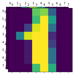
[ 0. 0. 6. 13. 10. 0. 0. 0.]]このデータを表示してみるとこんな感じ。
<セル3>

plt.imshow(digits.images[0])

実行結果
またRGB(Red:赤、Green:緑、Blue:青の三元色で色を示す方法)やRGBA(先ほどのRGBに透過率αを加えたもの)でも入力することができます。
その場合は数値のところがさらに3つか4つの数字が含まれたリストになります。
RGBの場合はこんな感じ(データは適当に作りました)。
<セル4>

rgb = [[[100, 200, 50],[50, 100, 150],[200, 250, 100]],
       [[200, 200, 200],[100, 100, 100],[50, 50, 50]],
       [[100, 50, 50], [200, 100, 100], [50, 100, 100]]]

plt.imshow(rgb)

実行結果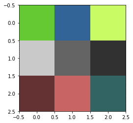
RGBAだとこんな感じ。
<セル5>

rgba = [[[100, 200, 50, 250],[50, 100, 150, 50],[200, 250, 100, 10]],
       [[200, 200, 200, 25],[100, 100, 100, 125],[50, 50, 50, 225]],
       [[100, 50, 50, 150], [200, 100, 100, 100], [50, 100, 100, 50]]]

plt.imshow(rgba)

実行結果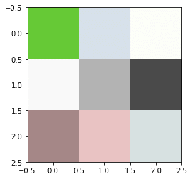
RGB、RGBAでは256段階の色調を操作でき、数値の範囲は0から255です。
cmap:使用するカラーマップ
先ほど入力できるデータは、二次元リストに色の強弱を示す数値が入っているものとRGB、もしくはRGBAの3種類があるとお話ししました。
RGBとRGBAに関しては色そのものを指定する形式なのですが、最初の二次元リストに色の強弱を示す数値が入っている形式では、色そのものは指定されていません。
つまりこの場合、どの数値がどの色を示すのか指定できる(指定しなければいけない)ことになります。
その際使用するのがカラーマップと呼ばれるものです。
Matplotlibで使用できるカラーマップはこちらを参照してください。
ちなみにデフォルトのカラーマップは「viridis」です。
つまり何もcmapの指定をしないこの場合は「viridis」。
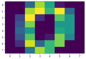
<セル6>

plt.imshow(digits.images[0])

実行結果
例えば「Reds」 を指定してみるとこんな感じ。
<セル7>

plt.imshow(digits.images[0], cmap="Reds")

実行結果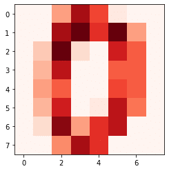
「coolwarm」を指定してみるとこんな感じ。
<セル8>

plt.imshow(digits.images[0], cmap="coolwarm")

実行結果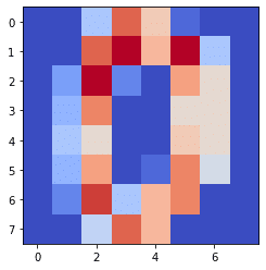
ということで色々試してしっくりくるものを見つけてみてください。
alpha:透明度
alphaは出力される図の透明度を小数で指定できます。
<セル9>

plt.imshow(digits.images[0], alpha=0.5)

実行結果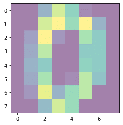
ぱっと見、全体が白くモヤがかかった感じになっていますが、多分これで50%透明化されているのだと思います。
次回は「vmax, vmin」「aspect」、「origin」に関して解説をしていきます。
ではでは今回はこんな感じで。
コメント