機械学習ライブラリScikit-learn
前回、機械学習ライブラリScikit-learnの糖尿病患者のデータセットを使い、Lassoモデルのオプションを試してみました。
今回は同様にElasticNetモデルのオプションを試していきましょう。
まずはデータの読み込みから。
<セル1>

from sklearn.datasets import load_diabetes
import pandas as pd

diabetes = load_diabetes()

df = pd.DataFrame(diabetes.data, columns=diabetes.feature_names)

df["target"] = diabetes.target

df

実行結果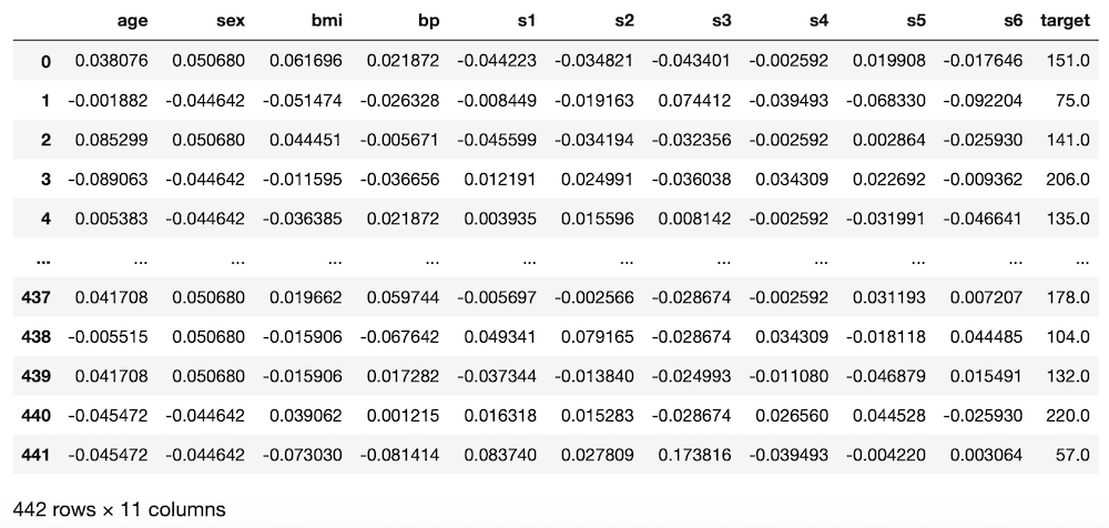
次に機械学習に用いる特徴量とターゲットをそれぞれ変数xとyに格納します。
(後で気付いたのですが、前の記事では「s6」も関連性がありそうということでしたが、忘れてしまいました。他の記事でも上記の組み合わせで行っているものもありますが、忘れたんだなぁと思って読んでください。)
<セル2>

x = df.loc[:, ["bmi", "s5", "bp", "s4", "s3"]]
y = df.loc[:, "target"]

実行結果
そしてElasticNetモデルを読み込んで、いつも通り100回試行した後、その予想精度のスコアの平均値を表示します。
その際、過学習になっていないか確認するため、テスト用データでのスコアだけでなく、学習用データでのスコアも計算します。
<セル3>

from sklearn.model_selection import train_test_split
from sklearn.linear_model import ElasticNet
from sklearn.metrics import r2_score
import numpy as np

trial = 100

pred_en_score = []; pred_en_train_score = []

for i in range(trial):
    x_train_ori, x_test_ori, y_train_ori, y_test_ori = train_test_split(x, y, test_size=0.2, train_size=0.8)

    model_en = ElasticNet()
    model_en.fit(x_train_ori, y_train_ori)
    pred_en_ori = model_en.predict(x_test_ori)
    pred_en_score.append(r2_score(y_test_ori, pred_en_ori))

    pred_en_ori_train = model_en.predict(x_train_ori)
    pred_en_train_score.append(r2_score(y_train_ori, pred_en_ori_train))

pred_en_ave = np.average(np.array(pred_en_score))
pred_en_train_ave = np.average(np.array(pred_en_train_score))

print(pred_en_ave, pred_en_train_ave)

実行結果
-0.00840863612850006 0.0077880822083276876
今回はかなり悪い予想精度になってしまっています。
オプションを変えることでこれが良くなるのでしょうか。
あとは最後の学習で得られたデータのグラフ表示もしてみましょう。
<セル4>

from matplotlib import pyplot as plt

fig=plt.figure(figsize=(8,6))
plt.clf()

plt.scatter(y_test_ori, pred_en_ori)

実行結果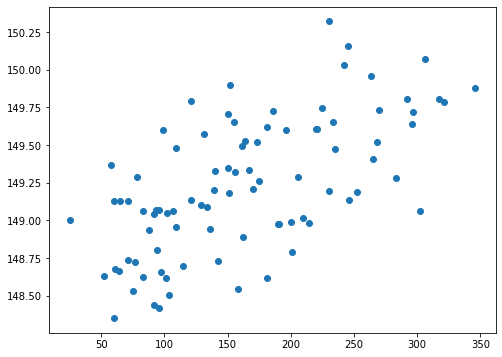
X軸に正解値、Y軸に予想値をとっていますので、右肩上がりのグラフになれば、正解に近いということ。
今回の結果もなんとなくですが、右肩上がりに見える…と思ったのですが、X軸とY軸の値が違いすぎるのが問題です。
X軸の範囲は0から350くらいですが、Y軸の値は148.00から150.50くらい。
これではスコアも悪いわけですね。
ElasticNetモデルのヘルプ
次にElasticNetモデルのヘルプを確認しておきましょう。
<セル5>

help(ElasticNet())

実行結果
Help on ElasticNet in module sklearn.linear_model._coordinate_descent object:

class ElasticNet(sklearn.base.MultiOutputMixin, sklearn.base.RegressorMixin, sklearn.linear_model._base.LinearModel)
 |  ElasticNet(alpha=1.0, *, l1_ratio=0.5, fit_intercept=True, normalize=False, precompute=False, max_iter=1000, copy_X=True, tol=0.0001, warm_start=False, positive=False, random_state=None, selection='cyclic')
 |
 |  Linear regression with combined L1 and L2 priors as regularizer.
 |
 |  Minimizes the objective function::
 |
 |          1 / (2 * n_samples) * ||y - Xw||^2_2
 |          + alpha * l1_ratio * ||w||_1
 |          + 0.5 * alpha * (1 - l1_ratio) * ||w||^2_2
 |
 |  If you are interested in controlling the L1 and L2 penalty
 |  separately, keep in mind that this is equivalent to::
 |
 |          a * L1 + b * L2
(中略)
 |  Parameters
 |  ----------
 |  alpha : float, default=1.0
 |      Constant that multiplies the penalty terms. Defaults to 1.0.
 |      See the notes for the exact mathematical meaning of this
 |      parameter. ``alpha = 0`` is equivalent to an ordinary least square,
 |      solved by the :class:`LinearRegression` object. For numerical
 |      reasons, using ``alpha = 0`` with the ``Lasso`` object is not advised.
 |      Given this, you should use the :class:`LinearRegression` object.
 |
 |  l1_ratio : float, default=0.5
 |      The ElasticNet mixing parameter, with ``0 <= l1_ratio <= 1``. For
 |      ``l1_ratio = 0`` the penalty is an L2 penalty. ``For l1_ratio = 1`` it
 |      is an L1 penalty.  For ``0 < l1_ratio < 1``, the penalty is a
 |      combination of L1 and L2.
 |
 |  fit_intercept : bool, default=True
 |      Whether the intercept should be estimated or not. If ``False``, the
 |      data is assumed to be already centered.
 |
 |  normalize : bool, default=False
 |      This parameter is ignored when ``fit_intercept`` is set to False.
 |      If True, the regressors X will be normalized before regression by
 |      subtracting the mean and dividing by the l2-norm.
 |      If you wish to standardize, please use
 |      :class:`sklearn.preprocessing.StandardScaler` before calling ``fit``
 |      on an estimator with ``normalize=False``.
 |
 |  precompute : bool or array-like of shape (n_features, n_features),                 default=False
 |      Whether to use a precomputed Gram matrix to speed up
 |      calculations. The Gram matrix can also be passed as argument.
 |      For sparse input this option is always ``True`` to preserve sparsity.
 |
 |  max_iter : int, default=1000
 |      The maximum number of iterations
 |
 |  copy_X : bool, default=True
 |      If ``True``, X will be copied; else, it may be overwritten.
 |
 |  tol : float, default=1e-4
 |      The tolerance for the optimization: if the updates are
 |      smaller than ``tol``, the optimization code checks the
 |      dual gap for optimality and continues until it is smaller
 |      than ``tol``.
 |
 |  warm_start : bool, default=False
 |      When set to ``True``, reuse the solution of the previous call to fit as
 |      initialization, otherwise, just erase the previous solution.
 |      See :term:`the Glossary <warm_start>`.
 |
 |  positive : bool, default=False
 |      When set to ``True``, forces the coefficients to be positive.
 |
 |  random_state : int, RandomState instance, default=None
 |      The seed of the pseudo random number generator that selects a random
 |      feature to update. Used when ``selection`` == 'random'.
 |      Pass an int for reproducible output across multiple function calls.
 |      See :term:`Glossary <random_state>`.
 |
 |  selection : {'cyclic', 'random'}, default='cyclic'
 |      If set to 'random', a random coefficient is updated every iteration
 |      rather than looping over features sequentially by default. This
 |      (setting to 'random') often leads to significantly faster convergence
 |      especially when tol is higher than 1e-4.
ElasticNetモデルでは、「alpha」、「l1_ratio」、「fit_intercept」、「normalize」、「precompute」、「copy_x」、「max_iter」、「tol」、「warm_start」、「positive」、「random_state」、「selection」というオプションがあるようです。
今回は特に予想精度に関わりそうな「alpha」、「l1_ratio」に関していじってみましょう。
ちなみにヘルプと同様に解説はこちらのページでもみることができます。

alpha
alpha: Lassoモデル同様ElasticNetモデルでは正則化と呼ばれるパラメータの学習に制限をかけ、過学習を防ぐ仕組みがある。alphaはその制限をかけるための係数。
float値(小数)、デフォルト値は1.0
デフォルトが1.0なので、制限を強くかける方としてalphaを10に、制限を緩くする方としてalphaを0.1にしてみましょう。
それぞれ「model_en = ElasticNet(alpha=10)」、「model_en = ElasticNet(alpha=0.1)」として機械学習モデルを作成し、学習させます。
まずはalpha=10から。
<セル6 alpha=10>

trial = 100

pred_en_score = []; pred_en_train_score = []

for i in range(trial):
    x_train, x_test, y_train, y_test = train_test_split(x, y, test_size=0.2, train_size=0.8)

    model_en = ElasticNet(alpha=10)
    model_en.fit(x_train, y_train)
    pred_en = model_en.predict(x_test)
    pred_en_score.append(r2_score(y_test, pred_en))

    pred_en_train = model_en.predict(x_train)
    pred_en_train_score.append(r2_score(y_train, pred_en_train))

pred_en_ave = np.average(np.array(pred_en_score))
pred_en_train_ave = np.average(np.array(pred_en_train_score))

print(pred_en_ave, pred_en_train_ave)

実行結果
-0.015099578097767432 0.0
予想精度のスコアは「-0.015100」とより悪くなってしまいました。
fig=plt.figure(figsize=(8,6))
plt.clf()

plt.scatter(y_test_ori, pred_en_ori)
plt.scatter(y_test, pred_en)

実行結果
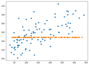
青点がalphaの設定なし、橙点がalpha=10の結果です。
Lassoモデルの時と同様、制限を強くかけすぎて、予想値が一点に固まってしまいました。
次にalpha=0.1。
<セル6 alpha=0.1>

trial = 100

pred_en_score = []; pred_en_train_score = []

for i in range(trial):
    x_train, x_test, y_train, y_test = train_test_split(x, y, test_size=0.2, train_size=0.8)

    model_en = ElasticNet(alpha=0.1)
    model_en.fit(x_train, y_train)
    pred_en = model_en.predict(x_test)
    pred_en_score.append(r2_score(y_test, pred_en))

    pred_en_train = model_en.predict(x_train)
    pred_en_train_score.append(r2_score(y_train, pred_en_train))

pred_en_ave = np.average(np.array(pred_en_score))
pred_en_train_ave = np.average(np.array(pred_en_train_score))

print(pred_en_ave, pred_en_train_ave)

実行結果
0.07581482098361181 0.08856067834801275
予想精度のスコアは「0.07581」と良くなっています。
<セル7 alpha=0.1>

fig=plt.figure(figsize=(8,6))
plt.clf()

plt.scatter(y_test_ori, pred_en_ori)
plt.scatter(y_test, pred_en)

実行結果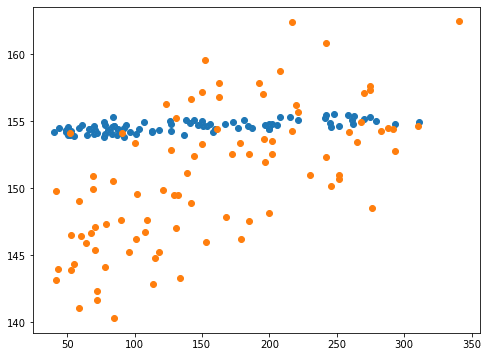
青点がalphaの設定なし、橙点がalpha=0.1の結果です。
Y軸の範囲が少し広がりましたが、X軸の範囲と比べるとまだまだ狭い範囲になっています。
ということでもうひとつ、alpha=0.01を試してみましょう。
<セル6 alpha=0.01>

trial = 100

pred_en_score = []; pred_en_train_score = []

for i in range(trial):
    x_train, x_test, y_train, y_test = train_test_split(x, y, test_size=0.2, train_size=0.8)

    model_en = ElasticNet(alpha=0.01)
    model_en.fit(x_train, y_train)
    pred_en = model_en.predict(x_test)
    pred_en_score.append(r2_score(y_test, pred_en))

    pred_en_train = model_en.predict(x_train)
    pred_en_train_score.append(r2_score(y_train, pred_en_train))

pred_en_ave = np.average(np.array(pred_en_score))
pred_en_train_ave = np.average(np.array(pred_en_train_score))

print(pred_en_ave, pred_en_train_ave)

実行結果
0.3476736634520542 0.3682683840927076
予想精度のスコアは「0.34767」と一気に良くなりました。
<セル7>

fig=plt.figure(figsize=(8,6))
plt.clf()

plt.scatter(y_test_ori, pred_en_ori)
plt.scatter(y_test, pred_en)

実行結果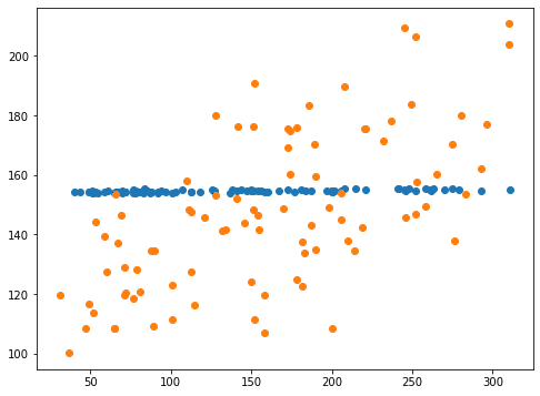
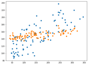
青点がalphaの設定なし、橙点がalpha=0.01の結果です。
予想値(Y軸方向)の範囲が広がり、正解値(X軸方向)の範囲に似通ってきました。
ただここで注意しなければいけないのは、ElasticNetモデルもLassoモデル同様、alphaを0にするとLinearRegressionモデルになるということです。
つまり今、alphaを0.01にしたということは、LinearRegressionモデルにかなり近くなったことを示しています。
そのため予想精度のスコアの向上はLinearRegressionモデルの予想精度に近づいたとみた方が良いでしょう。
ということはこのままalphaを下げていっても、LinearRegressionモデルの予想精度を超えることはないと考えられます。
l1_ratio
次は l1_ratioをいじっていきましょう。
L1、そしてL2というのがElasticNetモデルの特徴で、過学習を防ぐための「正則化項」というものらしいです。
このl1_ratioはL1とL2の項の比率を変えるオプションというわけです。
ちなみにLassoモデルとElasticNetモデル(そしてRidgeモデル)の違いを解説したサイトがあったので、紹介しておきますので、さらに知りたい方はぜひ行ってみてください。

ということで簡単な解説。
l1_ratio: ElasticNetモデルの正則化項L1、L2の比率を設定する。
float値(小数)、デフォルト値は0.5、設定範囲は0以上1以下。
範囲が0以上1以下ということで、まずは上限ギリギリの0.99にしてみましょう。
<セル8 l1_ratio=0.99>

trial = 100

pred_en_score = []; pred_en_train_score = []

for i in range(trial):
    x_train, x_test, y_train, y_test = train_test_split(x, y, test_size=0.2, train_size=0.8)

    model_en = ElasticNet(l1_ratio=0.99)
    model_en.fit(x_train, y_train)
    pred_en = model_en.predict(x_test)
    pred_en_score.append(r2_score(y_test, pred_en))

    pred_en_train = model_en.predict(x_train)
    pred_en_train_score.append(r2_score(y_train, pred_en_train))

pred_en_ave = np.average(np.array(pred_en_score))
pred_en_train_ave = np.average(np.array(pred_en_train_score))

print(pred_en_ave, pred_en_train_ave)

実行結果
0.127162151825194 0.14390151640382176
予想精度のスコアは「0.12716」と向上しました。
<セル9 l1_ratio=0.99>

fig=plt.figure(figsize=(8,6))
plt.clf()

plt.scatter(y_test_ori, pred_en_ori)
plt.scatter(y_test, pred_en)

実行結果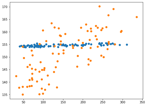
青点がl1_ratioの設定なし、橙点がl1_ratio=0.99の結果です。
予想値の幅が広がってはいますが、まだまだ正解値の幅に近付いていません。
ということで予想値と正解値のずれがスコアを落としている原因だと考えられます。
では次にl1_ratioを0.01にしてみましょう。
<セル8 l1_ratio=0.01>

trial = 100

pred_en_score = []; pred_en_train_score = []

for i in range(trial):
    x_train, x_test, y_train, y_test = train_test_split(x, y, test_size=0.2, train_size=0.8)

    model_en = ElasticNet(l1_ratio=0.01)
    model_en.fit(x_train, y_train)
    pred_en = model_en.predict(x_test)
    pred_en_score.append(r2_score(y_test, pred_en))

    pred_en_train = model_en.predict(x_train)
    pred_en_train_score.append(r2_score(y_train, pred_en_train))

pred_en_ave = np.average(np.array(pred_en_score))
pred_en_train_ave = np.average(np.array(pred_en_train_score))

print(pred_en_ave, pred_en_train_ave)

実行結果
-0.0074562451691631716 0.005409525832601795
こちらの場合はスコアが低くなってしまいました。
<セル9 l1_ratio=0.01>

fig=plt.figure(figsize=(8,6))
plt.clf()

plt.scatter(y_test_ori, pred_en_ori)
plt.scatter(y_test, pred_en)

実行結果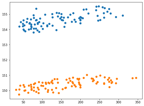
青点がl1_ratioの設定なし、橙点がl1_ratio=0.01の結果です。
こちらの場合は、予想値と正解値のずれは同じまま、つまり予想値の幅が小さいままで、予想値が下の方に平行移動した感じになっています。
これでは結局予想値と正解値は大きく異なるままなので、スコアは上がりません。
今回の結果としては、l1_ratioをL1側にする、つまり値を大きくすることで予想精度のスコアが向上しました。
これはalphaのようにLinearRegressionモデルに近づいたとかではなく、ElasticNetモデルの性質として、今回のデータに対してはl1_ratioをあげた方がいいということなのかなと考えています。
次回はRedgeRegressionのオプションを見てみることにしましょう。
ということで今回はこんな感じで。
コメント