機械学習ライブラリScikit-learn
前回、機械学習ライブラリScikit-learnの糖尿病患者のデータセットを使い、ElasticNetモデルのオプションを試してみました。
今回も同様にRidgeモデルのオプションを試していきましょう。
まずはデータの読み込みから。
<セル1>

from sklearn.datasets import load_diabetes
import pandas as pd

diabetes = load_diabetes()

df = pd.DataFrame(diabetes.data, columns=diabetes.feature_names)

df["target"] = diabetes.target

df

実行結果
次に機械学習に用いる特徴量とターゲットをそれぞれ変数xとyに格納します。
(後で気付いたのですが、前の記事では「s6」も関連性がありそうということでしたが、忘れてしまいました。他の記事でも上記の組み合わせで行っているものもありますが、忘れたんだなぁと思って読んでください。)
<セル2>

x = df.loc[:, ["bmi", "s5", "bp", "s4", "s3"]]
y = df.loc[:, "target"]

実行結果
そして今回はRidgeモデルを読み込んで、機械学習と予想を100回試した後、その予想精度のスコアの平均値を表示します。
その際、過学習になっていないか確認するため、テスト用データでのスコアだけでなく、学習用データでのスコアも計算します。
<セル3>

from sklearn.model_selection import train_test_split
from sklearn.linear_model import Ridge
from sklearn.metrics import r2_score
import numpy as np

trial = 100

pred_rd_score = []; pred_rd_train_score = []

for i in range(trial):
    x_train_ori, x_test_ori, y_train_ori, y_test_ori = train_test_split(x, y, test_size=0.2, train_size=0.8)

    model_rd = Ridge()
    model_rd.fit(x_train_ori, y_train_ori)
    pred_rd_ori = model_rd.predict(x_test_ori)
    pred_rd_score.append(r2_score(y_test_ori, pred_rd_ori))

    pred_rd_ori_train = model_rd.predict(x_train_ori)
    pred_rd_train_score.append(r2_score(y_train_ori, pred_rd_ori_train))

pred_rd_ave = np.average(np.array(pred_rd_score))
pred_rd_train_ave = np.average(np.array(pred_rd_train_score))

print(pred_rd_ave, pred_rd_train_ave)

実行結果
0.4094151872294987 0.4207727237569429
Ridgeモデルだとこれまでのモデル(LinearRegression、Lasso、ElasticNet)よりも良いスコアが出ました。
ということは今回のデータはRidgeモデルと相性がいいのでしょうか。
とりあえず最後の機械学習で得られたデータをグラフ化してみましょう。
<セル4>

from matplotlib import pyplot as plt

fig=plt.figure(figsize=(8,6))
plt.clf()

plt.scatter(y_test_ori, pred_rd_ori)

実行結果
X軸に正解値、Y軸に予想値をとっていますので、右肩上がりのグラフになれば、正解に近いということ。
なんとなく右肩上がりになっていて良い感じですが、X軸、Y軸の数値が少し違っているため、まだまだ正解にはたどり着けていないように思えます。
Ridgeモデルのヘルプ
ではRidgeモデルのヘルプを見てみましょう。
<セル5>

help(Ridge())

実行結果
Help on Ridge in module sklearn.linear_model._ridge object:

class Ridge(sklearn.base.MultiOutputMixin, sklearn.base.RegressorMixin, _BaseRidge)
 |  Ridge(alpha=1.0, *, fit_intercept=True, normalize=False, copy_X=True, max_iter=None, tol=0.001, solver='auto', random_state=None)

(中略)

 |  Parameters
 |  ----------
 |  alpha : {float, ndarray of shape (n_targets,)}, default=1.0
 |      Regularization strength; must be a positive float. Regularization
 |      improves the conditioning of the problem and reduces the variance of
 |      the estimates. Larger values specify stronger regularization.
 |      Alpha corresponds to ``1 / (2C)`` in other linear models such as
 |      :class:`~sklearn.linear_model.LogisticRegression` or
 |      :class:`sklearn.svm.LinearSVC`. If an array is passed, penalties are
 |      assumed to be specific to the targets. Hence they must correspond in
 |      number.
 |
 |  fit_intercept : bool, default=True
 |      Whether to fit the intercept for this model. If set
 |      to false, no intercept will be used in calculations
 |      (i.e. ``X`` and ``y`` are expected to be centered).
 |
 |  normalize : bool, default=False
 |      This parameter is ignored when ``fit_intercept`` is set to False.
 |      If True, the regressors X will be normalized before regression by
 |      subtracting the mean and dividing by the l2-norm.
 |      If you wish to standardize, please use
 |      :class:`sklearn.preprocessing.StandardScaler` before calling ``fit``
 |      on an estimator with ``normalize=False``.
 |
 |  copy_X : bool, default=True
 |      If True, X will be copied; else, it may be overwritten.
 |
 |  max_iter : int, default=None
 |      Maximum number of iterations for conjugate gradient solver.
 |      For 'sparse_cg' and 'lsqr' solvers, the default value is determined
 |      by scipy.sparse.linalg. For 'sag' solver, the default value is 1000.
 |
 |  tol : float, default=1e-3
 |      Precision of the solution.
 |
 |  solver : {'auto', 'svd', 'cholesky', 'lsqr', 'sparse_cg', 'sag', 'saga'},         default='auto'
 |      Solver to use in the computational routines:
 |
 |      - 'auto' chooses the solver automatically based on the type of data.
 |
 |      - 'svd' uses a Singular Value Decomposition of X to compute the Ridge
 |        coefficients. More stable for singular matrices than 'cholesky'.
 |
 |      - 'cholesky' uses the standard scipy.linalg.solve function to
 |        obtain a closed-form solution.
 |
 |      - 'sparse_cg' uses the conjugate gradient solver as found in
 |        scipy.sparse.linalg.cg. As an iterative algorithm, this solver is
 |        more appropriate than 'cholesky' for large-scale data
 |        (possibility to set `tol` and `max_iter`).
 |
 |      - 'lsqr' uses the dedicated regularized least-squares routine
 |        scipy.sparse.linalg.lsqr. It is the fastest and uses an iterative
 |        procedure.
 |
 |      - 'sag' uses a Stochastic Average Gradient descent, and 'saga' uses
 |        its improved, unbiased version named SAGA. Both methods also use an
 |        iterative procedure, and are often faster than other solvers when
 |        both n_samples and n_features are large. Note that 'sag' and
 |        'saga' fast convergence is only guaranteed on features with
 |        approximately the same scale. You can preprocess the data with a
 |        scaler from sklearn.preprocessing.
 |
 |      All last five solvers support both dense and sparse data. However, only
 |      'sag' and 'sparse_cg' supports sparse input when `fit_intercept` is
 |      True.
 |
 |      .. versionadded:: 0.17
 |         Stochastic Average Gradient descent solver.
 |      .. versionadded:: 0.19
 |         SAGA solver.
 |
 |  random_state : int, RandomState instance, default=None
 |      Used when ``solver`` == 'sag' or 'saga' to shuffle the data.
 |      See :term:`Glossary <random_state>` for details.
 |
 |      .. versionadded:: 0.17
 |         `random_state` to support Stochastic Average Gradient.
Ridgeモデルのパラメータとしては、「alpha」、「fit_intercept」、「normalize」、「copy_X」、「max_iter」、「tol」、「solver」、「random_state」といったオプションがあるようです。
今回は「alpha」と初めて出てきた「solver」をいじってみましょう。
ちなみにヘルプと同様に解説はこちらのページでもみることができます。

alpha
alpha: 正則化と呼ばれるパラメータの学習に制限をかけ、過学習を防ぐ仕組みがある。alphaはその制限をかけるための係数。値が大きくなるほど、制限が強くなる。
float値(小数)、デフォルト値は1.0
デフォルトが1.0なので、制限を強くかける方としてalphaを10に、制限を緩くする方としてalphaを0.1にしてみましょう。
ということで「model_rd = Ridge(alpha=10)」、「model_rd = Ridge(alpha=0.1)」として機械学習モデルを作成し、学習させます。
まずはalpha=10から。
<セル6 alpha=10>
trial = 100
pred_rd_score = []; pred_rd_train_score = []
for i in range(trial):
x_train, x_test, y_train, y_test = train_test_split(x, y, test_size=0.2, train_size=0.8)
model_rd = Ridge(alpha=10)
model_rd.fit(x_train, y_train)
pred_rd = model_rd.predict(x_test)
pred_rd_score.append(r2_score(y_test, pred_rd))
pred_rd_train = model_rd.predict(x_train)
pred_rd_train_score.append(r2_score(y_train, pred_rd_train))
pred_rd_ave = np.average(np.array(pred_rd_score))
pred_rd_train_ave = np.average(np.array(pred_rd_train_score))
print(pred_rd_ave, pred_rd_train_ave)
実行結果
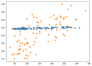
0.13064174595531175 0.14527286981830956alphaがデフォルト(1.0)の時の0.40942と比べ、0.13064と劇的に悪化してしまいました。
多分制限が強すぎて、値が収束しかかっているのではないでしょうか。
ということでグラフ表示してみましょう。
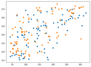
<セル7 alpha=10>

fig=plt.figure(figsize=(8,6))
plt.clf()

plt.scatter(y_test_ori, pred_rd_ori)
plt.scatter(y_test, pred_rd)

実行結果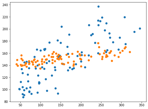
予想値がある一点に偏ってしまっています。
これが制限を強くかけ過ぎた状態だとみていいでしょう。
では次にalpha=0.1としてみます。
<セル6 alpha=0.1>

trial = 100

pred_rd_score = []; pred_rd_train_score = []

for i in range(trial):
    x_train, x_test, y_train, y_test = train_test_split(x, y, test_size=0.2, train_size=0.8)

    model_rd = Ridge(alpha=0.1)
    model_rd.fit(x_train, y_train)
    pred_rd = model_rd.predict(x_test)
    pred_rd_score.append(r2_score(y_test, pred_rd))

    pred_rd_train = model_rd.predict(x_train)
    pred_rd_train_score.append(r2_score(y_train, pred_rd_train))

pred_rd_ave = np.average(np.array(pred_rd_score))
pred_rd_train_ave = np.average(np.array(pred_rd_train_score))

print(pred_rd_ave, pred_rd_train_ave)

実行結果
0.46265714876109454 0.4933511689453928
alphaをデフォルト(1.0)の場合は0.40942だったのに比べ、alpha=0.1とすると0.46266と0.05程度も良くなりました。
学習用データセットを使った場合でも0.49335と特に過学習になっている様子はありません。
これはちょっと期待が持てるのかな。
グラフ表示をしてみましょう。
<セル7 alpha=0.1>

fig=plt.figure(figsize=(8,6))
plt.clf()

plt.scatter(y_test_ori, pred_rd_ori)
plt.scatter(y_test, pred_rd)

実行結果
思ったよりも良くなった感はグラフからは見えませんね。
全体的に少し上下にばらつきが増加している感じはしますが、右肩上がりっぷりはそれほどデフォルトと変わらないんじゃないかと思います。
Solver
Solver: Ridgeモデルを使う際の係数を算出するための計算方法を指定する(多分?)。
auto、svd、cholesky、lsqr、sparse_cg、sag、sagaから選択する。デフォルト値はauto
正直言って、このsolverがそれぞれどういう計算をしているのか私にはさっぱり分かりません。
とりあえずちょっと調べてみたので、リストにしておきます。
(ちなみに間違っているかもしれませんので、取扱注意!)
svd:Singular Value Decomposition(特異値分解)
cholesky: cholesky decomposition(コレスキー分解)
lsqr: regularized least-squares(正則化最小二乗法)
sparse_cg: sparse conjugate gradient (共役勾配法)

sag: stochastic gradient descent (確率的勾配降下法)
saga: unbiased version of stochastic gradient descent (バイアスのない確率的勾配降下法)

細かいことは全く分かりませんが、Ridgeモデルのあるパラメータを算出するための計算法が色々あって、それを変更するためのオプションだ考えられます。
ということでここからは試してみるのみ!
solver=”svd”
<セル8 solver="svd">

trial = 100

pred_rd_score = []; pred_rd_train_score = []

for i in range(trial):
    x_train, x_test, y_train, y_test = train_test_split(x, y, test_size=0.2, train_size=0.8)

    model_rd = Ridge(solver="svd")
    model_rd.fit(x_train, y_train)
    pred_rd = model_rd.predict(x_test)
    pred_rd_score.append(r2_score(y_test, pred_rd))

    pred_rd_train = model_rd.predict(x_train)
    pred_rd_train_score.append(r2_score(y_train, pred_rd_train))

pred_rd_ave = np.average(np.array(pred_rd_score))
pred_rd_train_ave = np.average(np.array(pred_rd_train_score))

print(pred_rd_ave, pred_rd_train_ave)

実行結果
0.41006584225587944 0.41988801975679324
<セル9 solver="svd">
fig=plt.figure(figsize=(8,6))
plt.clf()
plt.scatter(y_test_ori, pred_rd_ori)
plt.scatter(y_test, pred_rd)
実行結果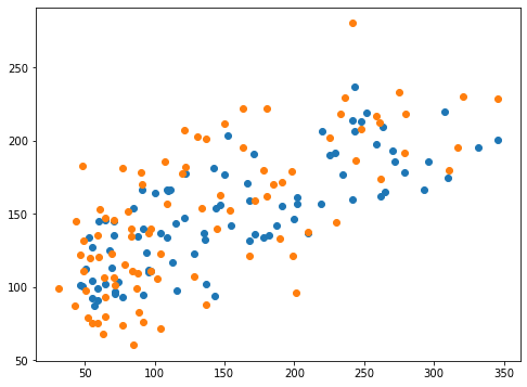
solver=”cholesky”
<セル8 solver="cholesky">

trial = 100

pred_rd_score = []; pred_rd_train_score = []

for i in range(trial):
    x_train, x_test, y_train, y_test = train_test_split(x, y, test_size=0.2, train_size=0.8)

    model_rd = Ridge(solver="cholesky")
    model_rd.fit(x_train, y_train)
    pred_rd = model_rd.predict(x_test)
    pred_rd_score.append(r2_score(y_test, pred_rd))

    pred_rd_train = model_rd.predict(x_train)
    pred_rd_train_score.append(r2_score(y_train, pred_rd_train))

pred_rd_ave = np.average(np.array(pred_rd_score))
pred_rd_train_ave = np.average(np.array(pred_rd_train_score))

print(pred_rd_ave, pred_rd_train_ave)

実行結果
0.4062048310329561 0.42233793298396094
<セル9 solver="cholesky">
fig=plt.figure(figsize=(8,6))
plt.clf()
plt.scatter(y_test_ori, pred_rd_ori)
plt.scatter(y_test, pred_rd)
実行結果
solver=”lsqr”
<セル8 solver="lsqr">

trial = 100

pred_rd_score = []; pred_rd_train_score = []

for i in range(trial):
    x_train, x_test, y_train, y_test = train_test_split(x, y, test_size=0.2, train_size=0.8)

    model_rd = Ridge(solver="lsqr")
    model_rd.fit(x_train, y_train)
    pred_rd = model_rd.predict(x_test)
    pred_rd_score.append(r2_score(y_test, pred_rd))

    pred_rd_train = model_rd.predict(x_train)
    pred_rd_train_score.append(r2_score(y_train, pred_rd_train))

pred_rd_ave = np.average(np.array(pred_rd_score))
pred_rd_train_ave = np.average(np.array(pred_rd_train_score))

print(pred_rd_ave, pred_rd_train_ave)

実行結果
0.41004199569597916 0.4202214331094112
<セル9 solver="lsqr">
fig=plt.figure(figsize=(8,6))
plt.clf()
plt.scatter(y_test_ori, pred_rd_ori)
plt.scatter(y_test, pred_rd)
実行結果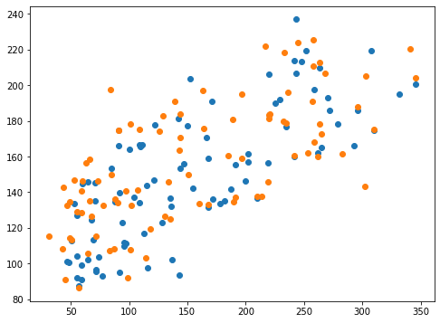
solver=”sparse_cg”
<セル8 solver="sparse_cg">

trial = 100

pred_rd_score = []; pred_rd_train_score = []

for i in range(trial):
    x_train, x_test, y_train, y_test = train_test_split(x, y, test_size=0.2, train_size=0.8)

    model_rd = Ridge(solver="sparse_cg")
    model_rd.fit(x_train, y_train)
    pred_rd = model_rd.predict(x_test)
    pred_rd_score.append(r2_score(y_test, pred_rd))

    pred_rd_train = model_rd.predict(x_train)
    pred_rd_train_score.append(r2_score(y_train, pred_rd_train))

pred_rd_ave = np.average(np.array(pred_rd_score))
pred_rd_train_ave = np.average(np.array(pred_rd_train_score))

print(pred_rd_ave, pred_rd_train_ave)

実行結果
0.4083775259681451 0.4211308435390734
<セル9 solver="sparse_cg">
fig=plt.figure(figsize=(8,6))
plt.clf()
plt.scatter(y_test_ori, pred_rd_ori)
plt.scatter(y_test, pred_rd)
実行結果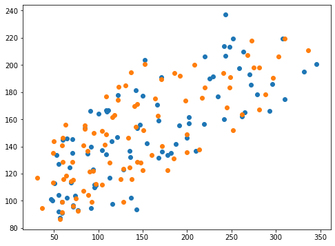
solver=”sag”
<セル8 solver="sag">

trial = 100

pred_rd_score = []; pred_rd_train_score = []

for i in range(trial):
    x_train, x_test, y_train, y_test = train_test_split(x, y, test_size=0.2, train_size=0.8)

    model_rd = Ridge(solver="sag")
    model_rd.fit(x_train, y_train)
    pred_rd = model_rd.predict(x_test)
    pred_rd_score.append(r2_score(y_test, pred_rd))

    pred_rd_train = model_rd.predict(x_train)
    pred_rd_train_score.append(r2_score(y_train, pred_rd_train))

pred_rd_ave = np.average(np.array(pred_rd_score))
pred_rd_train_ave = np.average(np.array(pred_rd_train_score))

print(pred_rd_ave, pred_rd_train_ave)

実行結果
0.40280066935984904 0.4220934440493007
<セル9 solver="sag">
fig=plt.figure(figsize=(8,6))
plt.clf()
plt.scatter(y_test_ori, pred_rd_ori)
plt.scatter(y_test, pred_rd)
実行結果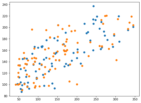
solver=”saga”
<セル8 solver="saga">

trial = 100

pred_rd_score = []; pred_rd_train_score = []

for i in range(trial):
    x_train, x_test, y_train, y_test = train_test_split(x, y, test_size=0.2, train_size=0.8)

    model_rd = Ridge(solver="saga")
    model_rd.fit(x_train, y_train)
    pred_rd = model_rd.predict(x_test)
    pred_rd_score.append(r2_score(y_test, pred_rd))

    pred_rd_train = model_rd.predict(x_train)
    pred_rd_train_score.append(r2_score(y_train, pred_rd_train))

pred_rd_ave = np.average(np.array(pred_rd_score))
pred_rd_train_ave = np.average(np.array(pred_rd_train_score))

print(pred_rd_ave, pred_rd_train_ave)

実行結果
0.407369467642637 0.4212855842690119
<セル9 solver="saga">
fig=plt.figure(figsize=(8,6))
plt.clf()
plt.scatter(y_test_ori, pred_rd_ori)
plt.scatter(y_test, pred_rd)
実行結果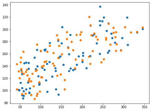
Solverまとめ
とりあえずそれぞれのSolverで得られたスコアを表にしてみました。
| Solver | テストデータセット | 訓練データセット |
| svd | 0.41007 | 0.41989 |
| cholesky | 0.40620 | 0.42234 |
| lsqr | 0.41004 | 0.42022 |
| sparse_cg | 0.40838 | 0.42113 |
| sag | 0.40280 | 0.42209 |
| saga | 0.40737 | 0.42129 |
正直に言うと、全く何かが変わった感じがしません。
もしかしたら今回のデータセットでは影響が出にくく、特殊なデータの時にのみ効果を発揮するなんてことがあるのかもしれません。
とりあえずSolverはautoにしておいて、ふと思い出した時に変えてみるくらいの気持ちでいいのかなと感じました。
次回はSVRのオプションを見ていくことにしましょう。
ということで今回はこんな感じで。
コメント